Case Study: Zebrafish pigementation

In our previous zebrafish tutorial, we have shown how dynamo goes beyond discrete RNA velocity vectors to continuous RNA vector field functions. In this tutorial, we will demonstrate a set of awesome downstream differential geometry and dynamical systems based analyses, enabled by the differentiable vector field functions, to gain deep functional and predictive insights of cell fate transition during zebrafish pigmentation (Saunders, et al. 2019).

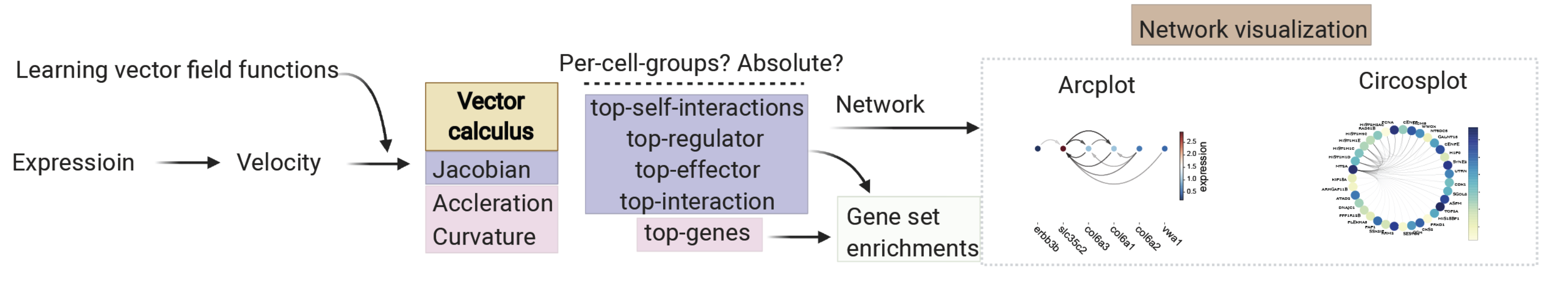
With differential geometry analysis of the continuous vector field functions, we can calculate the RNA Jacobian (see our primer on differential geometry), which is a cell by gene by gene tensor, encoding the gene regulatory network in each cell. With the Jacobian matrix, we can further derive the RNA acceleration, curvature, which are cell by gene matrices, just like gene expression dataset.

In general (see figure below), we can perform differential analyses and gene-set enrichment analyses based on top-ranked acceleration or curvature genes, as well as the top-ranked genes with the strongest self-interactions, top-ranked regulators/targets, or top-ranked interactions for each gene in individual cell types or across all cell types, with either raw or absolute values with the Jacobian tensor. Integrating that ranking information, we can build regulatory networks across different cell types, which can then be visualized with dynamo.pl.arcPlot(), dynamo.pl.circosPlot(), or other tools.

In this tutorial, we will cover following topics:

• learn continuous RNA velocity vector field functions in different spaces (e.g. umap or pca space)

• calculate RNA acceleration, curvature matrices (cell by gene)

• rank genes based on RNA velocity, curvature and acceleration matrices

• calculate RNA Jacobian tensor (cell by gene by gene) for genes with high PCA loadings.

• rank genes based on the jacobian tensor, which including:

• rank genes with strong positive or negative self-interaction (divergence ranking)

• other rankings, ranking modes including full_reg, full_eff, eff, reg and int

• build and visualize gene regulatory network with top ranked genes

• gene enrichment analyses of top ranked genes

• visualize Jacobian derived regulatory interactions across cells

• visualize gene expression, velocity, acceleration and curvature kinetics along pseudotime trajectory

• learn and visualize models of cell-fate transitions

Import relevant packages

import warnings
warnings.filterwarnings('ignore')
warnings.filterwarnings("ignore", message="numpy.dtype size changed")

import dynamo as dyn

dyn.configuration.set_figure_params('dynamo', background='white')
dyn.pl.style(font_path='Arial')
dyn.get_all_dependencies_version()

%load_ext autoreload
%autoreload 2

Using already downloaded Arial font from: /tmp/dynamo_arial.ttf
Registered custom font as: Arial


 ███                               ████████        
█████   █████    █████    █████    ███   █████      
   ██████   ██████   ██████   ████████      ████ 
  ___                           ████            ███
 |   \ _  _ _ _  __ _ _ __  ___                 ███
 | |) | || | ' \/ _` | '  \/ _ \█████           ███ 
 |___/ \_, |_||_\__,_|_|_|_\___/█████       ████  
       |__/                        ███   █████     
Tutorial: https://dynamo-release.readthedocs.io/       
                                     █████

package	umap-learn	typing-extensions	tqdm	statsmodels	setuptools	session-info	seaborn	scipy	requests	pynndescent	pre-commit	pandas	openpyxl	numdifftools	numba	networkx	mudata	matplotlib	loompy	leidenalg	igraph	dynamo-release	colorcet	anndata
version	0.5.7	4.13.2	4.67.1	0.14.4	79.0.0	1.0.1	0.13.2	1.11.4	2.32.3	0.5.13	4.2.0	2.2.3	3.1.5	0.9.41	0.60.0	3.4.2	0.3.1	3.10.3	3.0.8	0.10.2	0.11.8	1.4.2rc1	3.1.0	0.11.4

Set the logging level. Various logging level can be setted according to your needs:

• DEBUG: useful for dynamo development, show all logging information, including those debugging information

• INFO: useful for most dynamo users, show detailed dynamo running information

• WARNING: show only warning information

• ERROR: show only exception or error information

• CRITICAL: show only critical information

%matplotlib inline
from dynamo.dynamo_logger import main_info, LoggerManager
LoggerManager.main_logger.setLevel(LoggerManager.INFO)

Load processed data or data preprocessing

If you followed the zebrafish pigmentation tutorial, you can load the processed zebrafish adata object here for all downstream analysis.

adata = dyn.sample_data.zebrafish()
adata

|-----> Downloading data to ./data/zebrafish.h5ad
|-----> File ./data/zebrafish.h5ad already exists.

AnnData object with n_obs × n_vars = 4181 × 16940
    obs: 'split_id', 'sample', 'Size_Factor', 'condition', 'Cluster', 'Cell_type', 'umap_1', 'umap_2', 'batch'
    layers: 'spliced', 'unspliced'

preprocessor = dyn.pp.Preprocessor(cell_cycle_score_enable=True)
preprocessor.preprocess_adata(adata, recipe='monocle')
dyn.tl.dynamics(adata, cores=10)
dyn.tl.reduceDimension(adata)
dyn.tl.cell_velocities(adata)
dyn.tl.cell_velocities(adata)
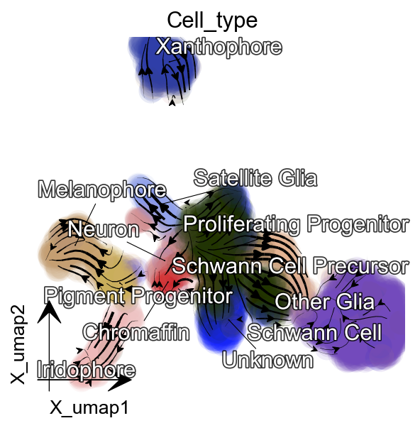
dyn.pl.streamline_plot(
    adata, color=['Cell_type'], 
    basis='umap', show_legend='on data', 
    s_kwargs_dict={'adjust_legend':True},
    show_arrowed_spines=False,
    figsize=(4,4),
)

|-----> Downloading data to ./data/zebrafish.h5ad
|-----> File ./data/zebrafish.h5ad already exists.
|-----> Running monocle preprocessing pipeline...
|-----------> filtered out 14 outlier cells
|-----------> filtered out 12746 outlier genes
|-----> PCA dimension reduction
|-----> <insert> X_pca to obsm in AnnData Object.
|-----> computing cell phase...
|-----> [Cell Phase Estimation] completed [49.3193s]
|-----> [Cell Cycle Scores Estimation] completed [0.5694s]
|-----> [Preprocessor-monocle] completed [4.0006s]
|-----> dynamics_del_2nd_moments_key is None. Using default value from DynamoAdataConfig: dynamics_del_2nd_moments_key=False
|-----------> removing existing M layers:[]...
|-----------> making adata smooth...
|-----> calculating first/second moments...
|-----> [moments calculation] completed [37.9759s]
|-----> retrieve data for non-linear dimension reduction...
|-----> [UMAP] using X_pca with n_pca_components = 30
|-----> <insert> X_umap to obsm in AnnData Object.
|-----> [UMAP] completed [12.8499s]
|-----> incomplete neighbor graph info detected: connectivities and distances do not exist in adata.obsp, indices not in adata.uns.neighbors.
|-----> Neighbor graph is broken, recomputing....
|-----> Start computing neighbor graph...
|-----------> X_data is None, fetching or recomputing...
|-----> fetching X data from layer:None, basis:pca
|-----> method arg is None, choosing methods automatically...
|-----------> method ball_tree selected
|-----> [calculating transition matrix via pearson kernel with sqrt transform.] in progress: 100.0000%|-----> [calculating transition matrix via pearson kernel with sqrt transform.] completed [6.0389s]
|-----> [projecting velocity vector to low dimensional embedding] in progress: 100.0000%|-----> [projecting velocity vector to low dimensional embedding] completed [1.1716s]
|-----> method arg is None, choosing methods automatically...
|-----------> method kd_tree selected
Using existing pearson_transition_matrix found in .obsp.
|-----> [projecting velocity vector to low dimensional embedding] in progress: 100.0000%|-----> [projecting velocity vector to low dimensional embedding] completed [1.1949s]
|-----> method arg is None, choosing methods automatically...
|-----------> method kd_tree selected
|-----> method arg is None, choosing methods automatically...
|-----------> method kd_tree selected
|-----------> plotting with basis key=X_umap
|-----------> skip filtering Cell_type by stack threshold when stacking color because it is not a numeric type

If you confronted errors when saving dynamo processed adata object, please see the very end of this tutorial.

If you would like to start from scratch, use the following code to preprocess the zebrafish adata object (or use your own dataset):

adata = dyn.sample_data.zebrafish()

dyn.pp.recipe_monocle(adata)
dyn.tl.dynamics(adata, cores=3)

dyn.tl.reduceDimension(adata)
dyn.tl.cell_velocities(adata)

dyn.tl.cell_velocities(adata)
dyn.pl.streamline_plot(adata, color=['Cell_type'])

Differential geometry analysis

In this part we will demonstrate how to leverage dynamo to estimate RNA jacobian (reveals state-dependent regulation), RNA acceleration/curvature (reveals earlier drivers and fate decision points), etc.

To gain functional and biological insights, we can perform a series of downstream analysis with the computed differential geometric quantities. We can first rank genes across all cells or in each cell group for any of those differential geometric quantities, followed by gene set enrichment analyses of the top ranked genes, as well as regulatory network construction and visualization.

The differential geometry and dynamical systems (i.e. fixed points, nullclines, etc mentioned in the previous zebrafish tutorial) are conventionally used to describe small-scale systems, while the vector field we build comes from high-dimensional genomics datasets. From this, you can appreciate that with dynamo, we are bridging small-scale systems-biology/physics type of thinking with high-dimensional genomics using ML, something really unimaginable until very recently!

In order to calculate RNA jacobian, acceleration and curvature, we can either learn the vector field function directly in the gene expression space or on the PCA space but then project the differential geometric quantities learned in PCA space back to the original gene expression space. Since we often have thousands of genes, we generally learn vector field in PCA space to avoid the curse of dimensionality and to improve the efficiency and accuracy of our calculation.

Vector field learning in PCA space

To learn PCA basis based RNA velocity vector field function, we need to first project the RNA velocities into PCA space.

dyn.tl.cell_velocities(adata, basis='pca');

Using existing pearson_transition_matrix found in .obsp.
|-----> [projecting velocity vector to low dimensional embedding] in progress: 100.0000%|-----> [projecting velocity vector to low dimensional embedding] completed [1.3163s]
|-----> method arg is None, choosing methods automatically...
|-----------> method kd_tree selected

Then we will use the dynamo.vf.VectorField() function to learn the vector field function in PCA space. This function relies on sparseVFC to learn the high dimensional vector field function in the entire expression space from sparse single cell velocity vector samples robustly.

Note that if you don’t provide any basis, vector field will be learned in the original gene expression and you can learn vector field for other basis too, as long as you have the RNA velocities projected in that basis.

Related information for the learned vector field are stored in adata.

dyn.vf.VectorField(
    adata, 
    basis='pca',
    M=100
)

|-----> VectorField reconstruction begins...
|-----> Retrieve X and V based on basis: PCA. 
        Vector field will be learned in the PCA space.
|-----> Learning vector field with method: sparsevfc.
|-----> [SparseVFC] begins...
|-----> Sampling control points based on data velocity magnitude...
|-----> method arg is None, choosing methods automatically...
|-----------> method ball_tree selected
|-----> [SparseVFC] completed [1.2615s]
|-----> [VectorField] completed [1.4585s]

Velocity, acceleration and curvature ranking

To gain functional insights of the biological process under study, we design a set of ranking methods to rank gene’s absolute, positive, negative vector field quantities in different cell groups that you can specify. Here we will first demonstrate how to rank genes based on their velocity matrix.

Basically, the rank functions in the vector field submodule (dynamo.vf) of dynamo is organized as rank_{quantities}_genes where {quantities} can be any differential geometry quantities, including, velocity, divergence, acceleration, curvature, jacobian:

• dynamo.vf.rank_velocity_genes()(adata, groups=’Cell_type’)

• dynamo.vf.rank_divergence_genes()(adata, groups=’Cell_type’)

• dynamo.vf.rank_acceleration_genes()(adata, groups=’Cell_type’)

• dynamo.vf.rank_curvature_genes()(adata, groups=’Cell_type’)

• dynamo.vf.rank_jacobian_genes()(adata, groups=’Cell_type’)

Gene ranking for different quantities (except jacobian, see below) are done based on both their raw and absolute velocities for each cell group when groups is set or for all cells if it is not set.

dyn.vf.rank_velocity_genes(adata, 
                           groups='Cell_type', 
                           vkey="velocity_S");

Ranking results are saved in .uns with the pattern rank_{quantities}genes or **rank_abs{quantities}_genes** where {quantities} can be any differential geometry quantities and the one with _abs indicates the ranking is based on absolute values instead of raw values.

We can save the speed ranking information to rank_speed or rank_abs_speed for future usages if needed.

rank_speed = adata.uns['rank_velocity_S'];
rank_abs_speed = adata.uns['rank_abs_velocity_S'];

Next we use dynamo.vf.acceleration() to compute acceleration for each cell with the learned vector field in adata. Note that we use PCA basis to calculate acceleration, but dynamo.vf.acceleration() will by default project acceleration_pca back to the original high dimension gene-wise space. You can check the resulted adata which will have both acceleration (in .layers) and acceleration_pca (in .obsm). We can also rank acceleration in the same fashion as what we did to velocity.

dyn.vf.acceleration(adata, basis='pca')

|-----> [Calculating acceleration] in progress: 100.0000%|-----> [Calculating acceleration] completed [0.1735s]

dyn.vf.rank_acceleration_genes(adata, 
                               groups='Cell_type', 
                               akey="acceleration", 
                               prefix_store="rank");
rank_acceleration = adata.uns['rank_acceleration'];
rank_abs_acceleration = adata.uns['rank_abs_acceleration'];

Similarly, we can also use dynamo.vf.curvature() to calculate curvature for each cell with the reconstructed vector field function stored in adata. dynamo.vf.rank_curvature_genes() ranks genes based on their raw or absolute curvature values in different cell groups.

dyn.vf.curvature(adata, basis='pca');

|-----> [Calculating acceleration] in progress: 100.0000%|-----> [Calculating acceleration] completed [0.1499s]
|-----> [Calculating curvature] in progress: 100.0000%|-----> [Calculating curvature] completed [0.1522s]

dyn.vf.rank_curvature_genes(adata, groups='Cell_type');

Now we estimated RNA acceleration and RNA curvature, we can visualize the acceleration or curvature for individual genes just like what we can do with gene expression or velocity, etc.

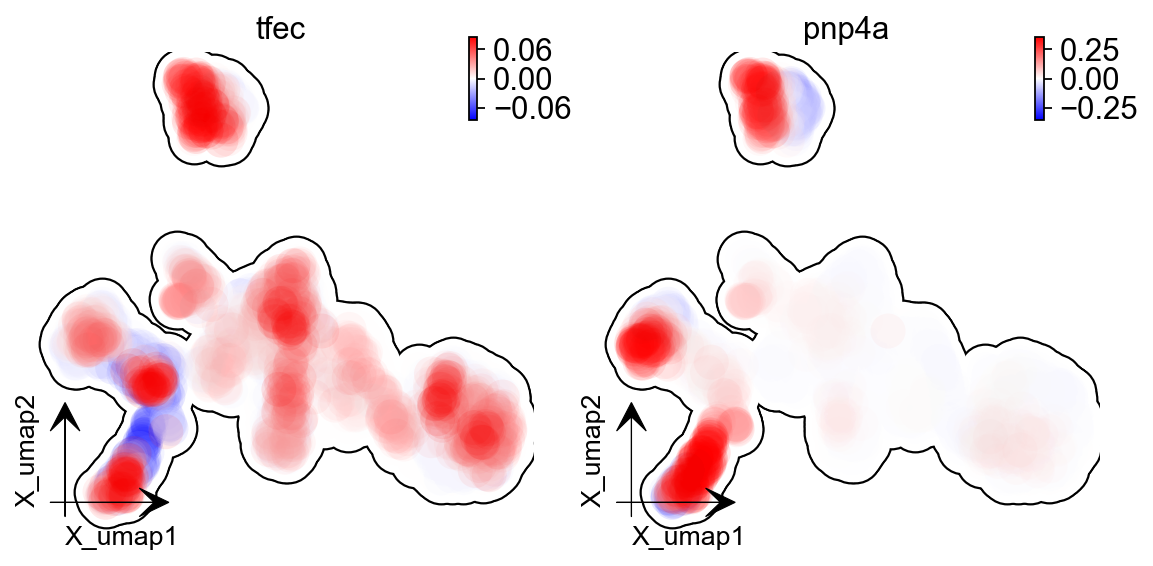
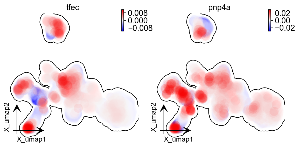
Let us show the velocity for gene tfec and pnp4a. bwr (blue-white-red) colormap is used here because velocity has both positive and negative values. The same applies to acceleration and curvature.

dyn.pl.umap(adata, color=['tfec', 'pnp4a'], 
            layer='velocity_S', frontier=True,
           figsize=(5,4),dpi=80)

|-----------> plotting with basis key=X_umap
|-----------> plotting with basis key=X_umap

This is for acceleration of genes tfec and pnp4a.

dyn.pl.umap(adata, color=['tfec', 'pnp4a'], 
            layer='acceleration', frontier=True,
           figsize=(5,4),dpi=80)

|-----------> plotting with basis key=X_umap
|-----------> plotting with basis key=X_umap

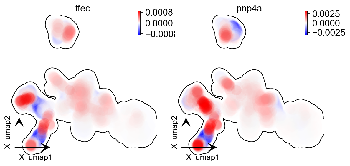
This is for curvature of genes tfec and pnp4a.

dyn.pl.umap(adata, color=['tfec', 'pnp4a'], 
            layer='curvature', frontier=True,
           figsize=(5,4),dpi=80)

|-----------> plotting with basis key=X_umap
|-----------> plotting with basis key=X_umap

The purpose for us to develop vaious differential geometry analyses is to derive functional predictions. So let us work on this a little bit next.

Gene set enrichment

In this section, we show our first approach to reveal functional insights with the dynamo.ext.enrichr() function implemented in dynamo, a python wrapper for Enrichr, to identify biological pathways with statistical significance.

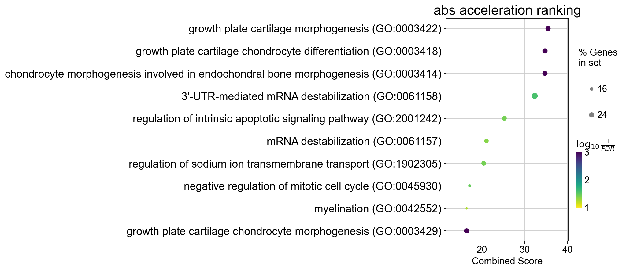
We noticed that the previous study (Saunders, et al. 2019) reported a “unknown” cell type from their conventional markers based cell-typing method based on total RNA expression levels. We wonder whether we can unveil its cell-type identify with dynamo. Therefore, we perform gene set enrichment analysis with the top-ranked genes with the highest absolute acceleration from this previously “unknown” cell type. Interestingly, we found the genes were enriched in chondrocyte-related pathways, indicative of a potential chondrocytic origin.

enr = dyn.ext.enrichr(adata.uns['rank_abs_acceleration']['Unknown'][:250].to_list(), 
                      organism='Fish', outdir='./enrichr', 
                      gene_sets='GO_Biological_Process_2018')

from gseapy.plot import barplot, dotplot
dotplot(enr.res2d, title='abs acceleration ranking', cmap='viridis_r', cutoff=0.1)

<Axes: title={'center': 'abs acceleration ranking'}, xlabel='Combined Score'>

Jacobian Calculation and Ranking

Next we will calculate Jacobian for each cell with the reconstructed vector field. If we use PCA space, dynamo.vf.jacobian() can project the low dimension Jacobian results back to high dimension to get a cell by gene by gene tensor. You can check the jacobian_gene key from the .uns["jacobian_pca"] dictionary in the resulted adata object to confirm this.

The cell by gene by gene tensor is generally huge, especially for datasets with large number of cells. We thus would love to do some preprocessing to alleviate the burden of computational resource requirements, either by restricting the calculation to genes that have high loading in our pca analysis or by downsampling the cells that will be used to calculate the jacobian matrix in each cell.

For the first one, we will use dynamo.pp.top_pca_genes() to calculate top_pca_genes for adata, according to PCs loading in adata.uns. Note that n_top_genes below means we take the union of genes with top n absolute values for each principal components, so the resulting PCA genes may be larger than 100.

For the second one, we can use the following parameters in dynamo.vf.jacobian().

sampling=None,
sample_ncells=1000,

When the sampling is chosen from one of the 'random', 'velocity', 'trn', the function will sample sample_ncells according to the sampling method sample for the Jacobian matrix calculation in only sample_ncells sampled cells. We recommend dynamo users to start considering sampling cells with your adata object with more than 2500 cells while the top pca gene selected will be around 500.

dyn.pp.top_pca_genes(adata, n_top_genes=100)

AnnData object with n_obs × n_vars = 4167 × 16940
    obs: 'split_id', 'sample', 'Size_Factor', 'condition', 'Cluster', 'Cell_type', 'umap_1', 'umap_2', 'batch', 'nGenes', 'nCounts', 'pMito', 'pass_basic_filter', 'spliced_Size_Factor', 'initial_spliced_cell_size', 'initial_cell_size', 'unspliced_Size_Factor', 'initial_unspliced_cell_size', 'ntr', 'cell_cycle_phase', 'control_point_pca', 'inlier_prob_pca', 'obs_vf_angle_pca', 'acceleration_pca', 'curvature_pca'
    var: 'nCells', 'nCounts', 'pass_basic_filter', 'score', 'log_cv', 'log_m', 'frac', 'use_for_pca', 'ntr', 'use_for_dynamics', 'use_for_transition', 'top_pca_genes'
    uns: 'pp', 'velocyto_SVR', 'feature_selection', 'PCs', 'explained_variance_ratio_', 'pca_mean', 'cell_phase_order', 'cell_phase_genes', 'vel_params_names', 'dynamics', 'neighbors', 'umap_fit', 'grid_velocity_umap', 'Cell_type_colors', 'grid_velocity_pca', 'VecFld_pca', 'rank_velocity_S', 'rank_abs_velocity_S', 'rank_acceleration', 'rank_abs_acceleration', 'rank_curvature', 'rank_abs_curvature'
    obsm: 'X_pca', 'cell_cycle_scores', 'X_umap', 'velocity_umap', 'velocity_pca', 'velocity_pca_SparseVFC', 'X_pca_SparseVFC', 'acceleration_pca', 'curvature_pca'
    varm: 'vel_params'
    layers: 'spliced', 'unspliced', 'X_spliced', 'X_unspliced', 'M_u', 'M_uu', 'M_s', 'M_us', 'M_ss', 'velocity_S', 'acceleration', 'curvature'
    obsp: 'moments_con', 'distances', 'connectivities', 'pearson_transition_matrix'

Select top pca genes (flagged in top_pca_genes in .var after running pp.top_pca_genes) and use those genes to set the regulator/effectors that are necessary in cell-wise jacobian matrix calculation.

top_pca_genes = adata.var.index[adata.var.top_pca_genes];

Here we will ensure a set of the chondrocyte-related gene included in the Jacobian calculation so that we can visualize the regulatory network for those genes. You can include other set of genes you care about as long as they are genes used for pca dimension reduction, that is adata[:, genes].var.use_for_pca are all True.

top_pca_genes = ["erbb3b", "col6a3", "vwa1", "slc35c2", "col6a2", "col6a1"] + list(top_pca_genes)

dyn.vf.jacobian(adata, regulators=top_pca_genes, effectors=top_pca_genes);

We can take advantage of the cell-wise jacobian matrix to investigate gene regulation at single-cell resolution or a state-dependent fashion.

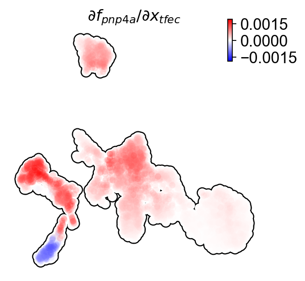
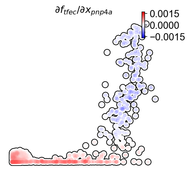
In iridophore cells, we found that pnp4a was potentially activated by tfec in the progenitors of iridophore lineage which is in line with that reported in Petratou et al. 2021. Futhermore, there seem to have a possible repression occurring when tfec expression level was high in the mature iridophore cells.

We can visualize the regulation from tfec to pnp4a (\(\frac{\partial f_{pnp4a}}{\partial f_{tfec}}\)) on the umap embedding. \(\frac{\partial f_{pnp4a}}{\partial f_{tfec}}\) denotes the effects of changing the expression of tfec to the velocity of pnp4a.

dyn.pl.jacobian(adata, regulators=['tfec'], 
                effectors=['pnp4a'], basis='umap',
               figsize=(4,4))

Similarly, we can also visualize the regulation from tfec to pnp4a (\(\frac{\partial f_{pnp4a}}{\partial f_{tfec}}\)) on top of the gene expression level of tfec (x-axis) to pnp4a (y-axis).

dyn.pl.jacobian(adata, regulators=['pnp4a'], effectors=['tfec'], 
                x='tfec', y="pnp4a", layer='M_s', basis='umap',
               figsize=(4,4))

Ranking for Jacobian matrices

After estimating the cell-wise Jacobian matrix, we now demonstrate different ways to rank genes based on the Jacobian matrix with dynamo.

We start with the so-called “divergence” ranking for each cell group. The “divergence” we are talking about here is different from the definition of divergence which is basically the sum of the diagonal elements of the Jacobian. Instead the divergence in this context points to the self-activation or self-inhibition terms.

The results of divergence ranking are stored in adata.uns['rank_div_gene_jacobian_pca'].

divergence_rank = dyn.vf.rank_divergence_genes(adata, groups='Cell_type');

divergence_rank.head()

	Chromaffin	Iridophore	Melanophore	Neuron	Other Glia	Pigment Progenitor	Proliferating Progenitor	Satellite Glia	Schwann Cell	Schwann Cell Precursor	Unknown	Xanthophore
0	mt2	tyrp1b	tspan36	mt2	tyrp1b	tyrp1b	tyrp1b	tuba8l3	plp1b	tyrp1b	ptmaa	si:ch211-251b21.1
1	mbpb	pmela	fosb	mbpb	plp1b	pmela	pmp22a	mt2	tyrp1b	pmela	mbpb	sdc4
2	mbpa	mt2	sdc4	gfap	pmela	pnp4a	ptmaa	tyrp1b	pmela	si:ch211-156j16.1	cldn19	wu:fc46h12
3	tyrp1b	gfap	fhl2a	mbpa	pmp22a	mt2	mbpa	pmp22a	MREG	pnp4a	mbpa	tspan36
4	pnp4a	mdkb	CRIP2	tyrp1b	gstp1	fhl2a	cldn19	tubb5	gstp1	mbpa	fstl3	tyrp1b

We can rank all other elements in the Jacobian. There are 5 parameters we provide in dynamo.vf.rank_jacobian_genes()’s argument list to rank the Jacobian:

• “full reg” or “full_reg”: top regulators are ranked for each effector for each cell group

• “full eff” or “full_reff”: top effectors are ranked for each regulator for each cell group

• “reg”: top regulators in each cell group

• “eff”: top effectors in each cell group

• “int”: top effector-regulator pairs in each cell group

Note that the default mode is “full reg”. More details can be found on API pages of online documentation. dynamo.vf.rank_jacobian_genes()

full_reg_rank = dyn.vf.rank_jacobian_genes(adata, 
                                           groups='Cell_type', 
                                           mode="full_reg", 
                                           abs=True, 
                                           output_values=True,
                                           return_df=True)

full_eff_rank = dyn.vf.rank_jacobian_genes(adata, 
                                           groups='Cell_type', 
                                           mode='full_eff', 
                                           abs=True, 
                                           exclude_diagonal=True, 
                                           output_values=True,
                                           return_df=True)

The results of full_eff and full_reg are dictionaries, whose keys are cluster (cell type in the case above) names and values are pd.DataFrame with rank information as well as coefficient values stored for each gene. See below:

type(full_reg_rank)

dict

print(full_reg_rank['Unknown'].shape)
full_reg_rank["Unknown"].head(2)

(467, 934)

	tmsb4x	tmsb4x_values	rplp2l	rplp2l_values	pvalb1	pvalb1_values	gfap	gfap_values	ptmab	ptmab_values	cotl1	cotl1_values	rpl37	rpl37_values	fosab	fosab_values	nfkbiab	nfkbiab_values	si:dkey-183i3.5	si:dkey-183i3.5_values	rpl36a	rpl36a_values	tlcd1	tlcd1_values	myo1cb	myo1cb_values	si:ch73-335m24.2	si:ch73-335m24.2_values	gpm6ab	gpm6ab_values	mbpb	mbpb_values	tp53inp1	tp53inp1_values	RPL41	RPL41_values	jupa	jupa_values	mbpa	mbpa_values	fstl1b	fstl1b_values	si:ch211-251b21.1	si:ch211-251b21.1_values	sdc4	sdc4_values	tuba8l4	tuba8l4_values	sparc	sparc_values	hmgb2a	hmgb2a_values	h3f3b.1	h3f3b.1_values	rpl38	rpl38_values	timp2a	timp2a_values	flj13639	flj13639_values	rplp1	rplp1_values	ptmaa	ptmaa_values	hmga1a	hmga1a_values	KRT	KRT_values	crip1	crip1_values	rgcc	rgcc_values	rtn3	rtn3_values	cd81a	cd81a_values	lgals2a	lgals2a_values	tfec	tfec_values	cox4i2	cox4i2_values	fstl3	fstl3_values	bzw1a	bzw1a_values	atf6	atf6_values	pmp22b	pmp22b_values	gstp1	gstp1_values	gch2	gch2_values	qdpra	qdpra_values	wu:fc46h12	wu:fc46h12_values	pnp5a	pnp5a_values	oca2	oca2_values	tyrp1a	tyrp1a_values	si:dkey-21a6.5	si:dkey-21a6.5_values	pfn2	pfn2_values	tyrp1b	tyrp1b_values	slc2a15b	slc2a15b_values	tspan36	tspan36_values	pmela	pmela_values	mlpha	mlpha_values	MREG	MREG_values	elovl1b	elovl1b_values	cyp2n13	cyp2n13_values	atp6ap2	atp6ap2_values	p4hb	p4hb_values	ppp1caa	ppp1caa_values	cd63	cd63_values	mcl1b	mcl1b_values	hmgn2	hmgn2_values	pmp22a	pmp22a_values	hsf2	hsf2_values	tuba8l3	tuba8l3_values	dynll1	dynll1_values	slc22a7a	slc22a7a_values	stmn4	stmn4_values	ctsba	ctsba_values	zgc:136930	zgc:136930_values	si:dkeyp-117h8.2	si:dkeyp-117h8.2_values	aldocb	aldocb_values	cd74a	cd74a_values	zgc:153704	zgc:153704_values	uraha	uraha_values	cfl1	cfl1_values	sept15	sept15_values	sncga	sncga_values	elovl1a	elovl1a_values	adka	adka_values	pnp4a	pnp4a_values	mt2	mt2_values	crabp1a	crabp1a_values	h2afvb	h2afvb_values	ak1	ak1_values	pef1	pef1_values	slc44a2	slc44a2_values	rhoub	rhoub_values	CYST	CYST_values	slc16a1a	slc16a1a_values	serinc1	serinc1_values	lim2.2	lim2.2_values	SHROOM2	SHROOM2_values	arl6ip1	arl6ip1_values	tubb4b	tubb4b_values	midn	midn_values	egr2b	egr2b_values	tubb5	tubb5_values	si:dkey-262k9.4	si:dkey-262k9.4_values	fxyd6l	fxyd6l_values	si:ch211-202a12.4	si:ch211-202a12.4_values	fhl2a	fhl2a_values	anxa2a	anxa2a_values	rasgef1ba	rasgef1ba_values	CRIP2	CRIP2_values	tpd52l1	tpd52l1_values	zgc:110699	zgc:110699_values	alx4a	alx4a_values	si:dkey-4e7.3	si:dkey-4e7.3_values	sox10	sox10_values	atp1b1a	atp1b1a_values	pcdh7a	pcdh7a_values	lgmn	lgmn_values	nrgna	nrgna_values	vat1	vat1_values	fa2h	fa2h_values	mdka	mdka_values	hmgb1a	hmgb1a_values	anxa13l	anxa13l_values	npc2	npc2_values	rap1b	rap1b_values	map1lc3b	map1lc3b_values	mdh1aa	mdh1aa_values	cmtm7	cmtm7_values	cirbpa	cirbpa_values	tpm3	tpm3_values	efhd1	efhd1_values	cdkn1bb	cdkn1bb_values	CABZ01032488.1	CABZ01032488.1_values	glrx	glrx_values	oacyl	oacyl_values	calm2a	calm2a_values	FBXO	FBXO_values	mcl1a	mcl1a_values	col4a1	col4a1_values	sepp1a	sepp1a_values	krt18	krt18_values	itm2ba	itm2ba_values	fez1	fez1_values	hsp90b1	hsp90b1_values	ehd2b	ehd2b_values	anxa5b	anxa5b_values	calm2b	calm2b_values	btg1	btg1_values	cd9b	cd9b_values	gapdhs	gapdhs_values	phlda2	phlda2_values	ip6k2a	ip6k2a_values	fosb	fosb_values	ugt8	ugt8_values	si:ch211-260e23.9	si:ch211-260e23.9_values	CR854824.1	CR854824.1_values	pleca	pleca_values	cx27.5	cx27.5_values	rnd3b	rnd3b_values	ndrg1a	ndrg1a_values	plekha1a	plekha1a_values	fxyd1	fxyd1_values	si:dkey-73n8.3	si:dkey-73n8.3_values	sema3b	sema3b_values	ninj2	ninj2_values	si:rp71-19m20.1	si:rp71-19m20.1_values	basp1	basp1_values	pbx4	pbx4_values	eno1a	eno1a_values	ctsd	ctsd_values	si:dkey-164f24.2	si:dkey-164f24.2_values	plp1b	plp1b_values	mpz	mpz_values	hmgb3a	hmgb3a_values	cd99l2	cd99l2_values	canx	canx_values	entpd1	entpd1_values	ndfip2	ndfip2_values	myo10l3	myo10l3_values	cldn19	cldn19_values	AKAP	AKAP_values	anxa3b	anxa3b_values	tjp2b	tjp2b_values	si:ch211-222l21.1	si:ch211-222l21.1_values	rpz5	rpz5_values	calm1b	calm1b_values	mdkb	mdkb_values	sox4a	sox4a_values	tuba8l	tuba8l_values	elavl4	elavl4_values	ddx6	ddx6_values	degs1	degs1_values	egr1	egr1_values	gdi1	gdi1_values	hsd11b1la	hsd11b1la_values	slc45a2	slc45a2_values	agtrap	agtrap_values	akap12a	akap12a_values	asmtl	asmtl_values	bnip3lb	bnip3lb_values	si:ch73-46j18.5	si:ch73-46j18.5_values	spry2	spry2_values	nfkbiaa	nfkbiaa_values	ccng1	ccng1_values	plecb	plecb_values	si:ch211-196l7.4	si:ch211-196l7.4_values	bscl2l	bscl2l_values	sgce	sgce_values	zdhhc2	zdhhc2_values	scarb1	scarb1_values	rtn1b	rtn1b_values	prtfdc1	prtfdc1_values	phyhd1	phyhd1_values	atic	atic_values	b2ml	b2ml_values	ngfrb	ngfrb_values	ndrg3a	ndrg3a_values	prdx1	prdx1_values	GABARAPL1	GABARAPL1_values	si:ch211-213a13.1	si:ch211-213a13.1_values	adipor2	adipor2_values	atf3	atf3_values	si:dkey-226k3.4	si:dkey-226k3.4_values	qki2	qki2_values	wls	wls_values	cldn7a	cldn7a_values	si:ch211-39i22.1	si:ch211-39i22.1_values	psap	psap_values	mgst1.2	mgst1.2_values	bace2	bace2_values	si:dkey-251i10.2	si:dkey-251i10.2_values	gch1	gch1_values	zgc:153031	zgc:153031_values	paics	paics_values	mcamb	mcamb_values	col14a1a	col14a1a_values	eif4ebp3l	eif4ebp3l_values	si:dkeyp-75h12.5	si:dkeyp-75h12.5_values	emc4	emc4_values	stard8	stard8_values	hbegfb	hbegfb_values	nr1d2a	nr1d2a_values	arhgef1b	arhgef1b_values	calm1a	calm1a_values	fabp3	fabp3_values	snap25a	snap25a_values	clstn2	clstn2_values	emp2	emp2_values	syngr2b	syngr2b_values	si:ch211-132g1.3	si:ch211-132g1.3_values	odc1	odc1_values	ythdf2	ythdf2_values	xbp1	xbp1_values	stmn2b	stmn2b_values	postna	postna_values	mef2cb	mef2cb_values	flna	flna_values	si:ch211-197g15.7	si:ch211-197g15.7_values	atp1a1b	atp1a1b_values	slc1a2b	slc1a2b_values	s100b	s100b_values	si:ch211-156j16.1	si:ch211-156j16.1_values	atp1a1a.1	atp1a1a.1_values	zgc:153012	zgc:153012_values	aatkb	aatkb_values	si:dkey-276j7.1	si:dkey-276j7.1_values	scn4ab	scn4ab_values	vcanb	vcanb_values	erbb3b	erbb3b_values	wasla	wasla_values	selt2	selt2_values	cdk1	cdk1_values	col6a3	col6a3_values	ppp1r15a	ppp1r15a_values	srsf5a	srsf5a_values	si:ch211-288g17.3	si:ch211-288g17.3_values	RAPGE	RAPGE_values	hoxb7a	hoxb7a_values	gpm6aa	gpm6aa_values	bhlhe40	bhlhe40_values	trib3	trib3_values	plpp3	plpp3_values	ahnak	ahnak_values	rrm2	rrm2_values	pdcd6	pdcd6_values	mad2l1	mad2l1_values	lfng	lfng_values	si:ch211-137a8.4	si:ch211-137a8.4_values	prrg4	prrg4_values	anxa4	anxa4_values	hepacama	hepacama_values	dedd1	dedd1_values	tuft1a	tuft1a_values	prdx5	prdx5_values	rtn1a	rtn1a_values	tmsb	tmsb_values	her4.2	her4.2_values	foxp4	foxp4_values	tagln2	tagln2_values	hapln1a	hapln1a_values	si:ch211-194k22.8	si:ch211-194k22.8_values	tcf3b	tcf3b_values	sncgb	sncgb_values	myl9b	myl9b_values	pcna	pcna_values	igfbp3	igfbp3_values	chp2	chp2_values	lbr	lbr_values	net1	net1_values	arrdc3b	arrdc3b_values	slc20a2	slc20a2_values	znf536	znf536_values	aif1l	aif1l_values	hmgn3	hmgn3_values	sncb	sncb_values	plpp1a	plpp1a_values	si:dkey-253d23.4	si:dkey-253d23.4_values	gulp1a	gulp1a_values	ivns1abpa	ivns1abpa_values	fam49a	fam49a_values	si:dkey-51a16.9	si:dkey-51a16.9_values	maptb	maptb_values	ccl19a.1	ccl19a.1_values	slc6a1b	slc6a1b_values	NAPSA	NAPSA_values	tspan10	tspan10_values	tmem176	tmem176_values	bco1	bco1_values	azin1a	azin1a_values	zgc:162150	zgc:162150_values	clu	clu_values	nfasca	nfasca_values	smox	smox_values	htra1a	htra1a_values	ubl3a	ubl3a_values	tspan2a	tspan2a_values	slc44a1b	slc44a1b_values	klf6a	klf6a_values	efna1b	efna1b_values	col6a2	col6a2_values	col6a1	col6a1_values	hmp19	hmp19_values	syt11a	syt11a_values	aatka	aatka_values	tmem125b	tmem125b_values	pcbp4	pcbp4_values	qkia	qkia_values	pfkfb4b	pfkfb4b_values	gpr143	gpr143_values	cntfr	cntfr_values	si:ch211-195b13.1	si:ch211-195b13.1_values	zgc:92242	zgc:92242_values	fam102ab	fam102ab_values	metrnl	metrnl_values	apodb	apodb_values	ppfibp1a	ppfibp1a_values	pik3ip1	pik3ip1_values	proza	proza_values	tspan7b	tspan7b_values	atp6v0cb	atp6v0cb_values	hspa5	hspa5_values	creb3l3l	creb3l3l_values	tmem59l	tmem59l_values	fkbp5	fkbp5_values	slc35c2	slc35c2_values	pisd	pisd_values	larp4ab	larp4ab_values	pax7b	pax7b_values	scn1ba	scn1ba_values	mtmr1b	mtmr1b_values	anxa13	anxa13_values	rbm24a	rbm24a_values	elovl6	elovl6_values	fosl1a	fosl1a_values	nr4a2b	nr4a2b_values	sb:cb81	sb:cb81_values	igf2bp3	igf2bp3_values	pdia6	pdia6_values	tspan15	tspan15_values	gldn	gldn_values	cmtm6	cmtm6_values	sypl2b	sypl2b_values	itga6b	itga6b_values	entpd3	entpd3_values	palm1b	palm1b_values	syt5a	syt5a_values	ALKB	ALKB_values	igfbp2a	igfbp2a_values	clstn1	clstn1_values	mknk2b	mknk2b_values	rab1ba	rab1ba_values	stmn2a	stmn2a_values	stx1b	stx1b_values	cdca7a	cdca7a_values	cdh11	cdh11_values	lmnb2	lmnb2_values	slc22a2	slc22a2_values	zgc:110789	zgc:110789_values	pcdh10a	pcdh10a_values	grasp	grasp_values	gnmt	gnmt_values	tfap2e	tfap2e_values	cadm4	cadm4_values	rhbdl3	rhbdl3_values	pik3r3a	pik3r3a_values	pah	pah_values	phyhiplb	phyhiplb_values	plk2b	plk2b_values	fstb	fstb_values	pdgfbb	pdgfbb_values	serinc5	serinc5_values	neurl1b	neurl1b_values	ctdsp2	ctdsp2_values	slc6a9	slc6a9_values	aqp1a.1	aqp1a.1_values	atp1b4	atp1b4_values	mmp17b	mmp17b_values	slc25a43	slc25a43_values	myo5b	myo5b_values	rab6ba	rab6ba_values	pcsk1nl	pcsk1nl_values	si:dkey-7j14.5	si:dkey-7j14.5_values	spock3	spock3_values	COL18	COL18_values	ttyh2l	ttyh2l_values	elavl3	elavl3_values	impdh1b	impdh1b_values	alcama	alcama_values	lrrc17	lrrc17_values	ston2	ston2_values	trpm1b	trpm1b_values	olfm1b	olfm1b_values	mcm6	mcm6_values	akap12b	akap12b_values	tsc22d2	tsc22d2_values	tcirg1a	tcirg1a_values	lhfpl2b	lhfpl2b_values	rnf13	rnf13_values	mical3a	mical3a_values	cyth1b	cyth1b_values	cpe	cpe_values	phgdh	phgdh_values	si:ch211-105c13.3	si:ch211-105c13.3_values	vwa1	vwa1_values	si:ch211-243a20.3	si:ch211-243a20.3_values	atp1b2a	atp1b2a_values	mki67	mki67_values	snap25b	snap25b_values	tfdp2	tfdp2_values	si:ch211-137i24.10	si:ch211-137i24.10_values	gpnmb	gpnmb_values	rdh5	rdh5_values	hells	hells_values	dct	dct_values	emp3b	emp3b_values	IFI	IFI_values	fam212aa	fam212aa_values	ponzr1	ponzr1_values	prph	prph_values	si:ch211-256m1.8	si:ch211-256m1.8_values	sytl2b	sytl2b_values	ccna2	ccna2_values	ddc	ddc_values	top2a	top2a_values	slc6a2	slc6a2_values
0	mbpa	0.001392	nfkbiab	0.001957	mcl1b	0.001208	si:ch211-222l21.1	0.001037	hmgn2	0.003338	cldn19	0.001032	mt2	0.001064	mt2	0.003449	mbpb	0.001441	nfkbiab	0.002291	mt2	0.001630	fstl3	0.000351	cldn19	0.001138	mbpb	0.000489	mbpb	0.001536	egr2b	0.003785	si:ch211-156j16.1	0.000668	mt2	0.001393	rgcc	0.000412	egr2b	0.003166	mbpb	0.000440	phlda2	0.001696	tyrp1b	0.000726	si:ch211-156j16.1	0.001881	mbpa	0.001603	hmgn2	0.006100	hmgn2	0.002982	mcl1b	0.000969	mbpb	0.001005	nfkbiab	0.000334	mt2	0.001473	ptmaa	0.002394	hmgn2	0.004448	hmgn2	0.001443	hmgb2a	0.002421	hmgb2a	0.003215	mbpb	0.000422	hmgb2a	0.002678	pnp4a	0.001228	fhl2a	0.000290	si:ch211-222l21.1	0.000384	mbpb	0.002465	p4hb	0.001673	mt2	0.000190	si:ch211-156j16.1	0.001475	mt2	0.001173	tyrp1b	0.001568	tyrp1b	0.000523	mcl1b	0.001566	wu:fc46h12	0.000535	tyrp1b	0.000532	tyrp1b	0.000723	wu:fc46h12	0.000764	rgcc	0.001457	tyrp1b	0.001869	wu:fc46h12	0.000597	wu:fc46h12	0.000888	tyrp1b	0.001654	wu:fc46h12	0.000521	tyrp1b	0.000950	mbpb	0.002098	hmgb2a	0.000814	anxa13l	0.000473	p4hb	0.001672	elovl1b	0.000374	mbpb	0.001856	mcl1b	0.003925	hmgn2	0.007998	si:ch211-137a8.4	0.003055	mcl1b	0.000452	mt2	0.002052	nfkbiab	0.002423	wu:fc46h12	0.000612	tubb5	0.000467	wu:fc46h12	0.000491	nfkbiab	0.001700	fstl3	0.000696	anxa13l	0.000782	nfkbiab	0.000510	si:dkey-183i3.5	0.001254	wu:fc46h12	0.000406	p4hb	0.001071	egr2b	0.000302	fstl3	0.001291	mbpa	0.001041	hmgn2	0.000365	pnp4a	0.001429	mt2	0.001699	si:ch211-222l21.1	0.000306	hmgn2	0.004269	tyrp1b	0.000482	pnp4a	0.000321	mbpb	0.000689	cldn19	0.000659	pnp4a	0.000403	fstl3	0.000187	mbpb	0.001053	ptmaa	0.000485	mbpa	0.000539	wu:fc46h12	0.000765	crip1	0.001509	fosab	0.000371	mbpa	0.001705	tubb5	0.001756	nrgna	0.000582	mbpa	0.000307	krt18	0.000680	pnp4a	0.001313	pnp4a	0.000424	mbpa	0.000864	pnp4a	0.001202	pnp4a	0.000493	pnp4a	0.000315	fhl2a	0.000346	pnp4a	0.000387	nfkbiab	0.001622	mt2	0.000862	nfkbiab	0.001266	mt2	0.000242	fstl3	0.001130	mbpb	0.000962	mbpb	0.000674	phlda2	0.002211	hmgn2	0.001058	mbpb	0.001263	mbpb	0.000715	mcl1b	0.001003	nfkbiab	0.000657	mcl1b	0.001051	dynll1	0.000322	hmgn2	0.001998	crip1	0.000338	mbpb	0.000939	rgcc	0.000954	fhl2a	0.000243	mt2	0.000460	wu:fc46h12	0.000262	nrgna	0.001038	nfkbiab	0.000397	plp1b	0.000681	mbpa	0.002136	hmgb2a	0.001059	mt2	0.002249	mbpb	0.002099	anxa13l	0.000462	mcl1b	0.000153	hmgb2a	0.000508	mt2	0.000706	crip1	0.001374	mbpa	0.001953	ptmaa	0.000303	mcl1b	0.000937	tubb4b	0.002317	pmp22b	0.001154	mt2	0.002139	mbpa	0.001016	si:ch211-156j16.1	0.001104	mbpb	0.000534	mbpb	0.000595	mbpb	0.000789	calm2b	0.000347	mbpb	0.001078	si:ch211-156j16.1	0.000674	fosab	0.000852	wu:fc46h12	0.000321	mbpb	0.000739	fstl3	0.000523	egr2b	0.001424	anxa13l	0.000558	si:dkey-183i3.5	0.000278	mcl1b	0.000373	crip1	0.000507	egr2b	0.000593	mcl1b	0.001114	mcl1b	0.000648	mcl1b	0.000831	anxa13l	0.000567	wu:fc46h12	0.000264	hmgb2a	0.003213	mbpb	0.000526	pmp22a	0.000737	cldn19	0.002369	mbpb	0.000425	mbpa	0.000732	cldn19	0.000378	mcl1b	0.002967	hmgb2a	0.001306	tubb5	0.000542	si:ch211-222l21.1	0.001181	pmp22a	0.001160	hmgn2	0.002230	tubb5	0.001340	mcl1b	0.000675	mbpa	0.000578	mt2	0.000657	anxa13l	0.000508	wu:fc46h12	0.000190	tyrp1b	0.000597	wu:fc46h12	0.000423	pnp4a	0.000857	ptmaa	0.000896	nfkbiab	0.000493	mbpb	0.000655	mbpa	0.000730	mt2	0.000634	mt2	0.000418	mbpa	0.000546	mbpa	0.000816	wu:fc46h12	0.000285	mbpb	0.000607	tyrp1b	0.000320	wu:fc46h12	0.000244	anxa13l	0.001106	wu:fc46h12	0.000203	wu:fc46h12	0.000152	rgcc	0.000304	mbpb	0.001185	hmgn2	0.000463	anxa13l	0.000634	mcl1b	0.000522	nfkbiab	0.000807	mbpb	0.000995	si:ch211-156j16.1	0.000246	dynll1	0.000718	pnp4a	0.000437	cldn19	0.001669	btg1	0.000238	si:ch211-222l21.1	0.000718	crip1	0.001031	si:ch211-156j16.1	0.000388	hmgb2a	0.000354	wu:fc46h12	0.000536	mcl1b	0.000469	wu:fc46h12	0.000271	mcl1b	0.000231	wu:fc46h12	0.000563	mbpa	0.000603	mbpb	0.000442	ptmaa	0.000421	anxa13l	0.000563	mbpa	0.000260	mbpa	0.000809	mbpb	0.000347	mbpb	0.000579	nfkbiab	0.001126	mbpa	0.002285	mt2	0.000983	mt2	0.000654	anxa13l	0.000410	rgcc	0.000607	cldn19	0.000258	mbpb	0.001905	nfkbiab	0.000983	fosab	0.000334	si:dkey-183i3.5	0.001267	tubb5	0.000800	hmgb2a	0.002129	hmgb2a	0.000760	phlda2	0.000487	mbpb	0.000461	hmgn2	0.000542	si:ch211-222l21.1	0.000579	cd81a	0.000518	phlda2	0.001922	nfkbiab	0.000487	si:ch211-156j16.1	0.000528	mbpb	0.00084	anxa13l	0.000686	si:ch211-137a8.4	0.002993	hmgb2a	0.000944	hmgb2a	0.000145	rgcc	0.000498	pmp22a	0.000627	hmgn2	0.001735	hmgb2a	0.000966	fosab	0.000298	plp1b	0.000672	hmgn2	0.002952	anxa13l	0.000331	mbpa	0.000410	anxa13l	0.000788	mcl1b	0.000798	mbpb	0.000278	mbpa	0.001042	fstl3	0.000508	hmgn2	0.002938	mbpa	0.000337	hmgn2	0.001063	hmgb2a	0.000611	nfkbiab	0.001359	mbpb	0.000739	mcl1b	0.000449	si:ch211-222l21.1	0.000292	mbpb	0.000515	mbpb	0.000723	nfkbiab	0.000515	anxa13l	0.000951	mt2	0.001198	mcl1b	0.000434	phlda2	0.002021	si:ch211-137a8.4	0.000661	hmgb2a	0.001569	anxa13l	0.000323	mcl1b	0.000291	mt2	0.000496	rgcc	0.000171	nfkbiab	0.002630	hmgb2a	0.000929	mbpb	0.000468	hmgn2	0.001575	fabp3	0.000159	si:ch211-156j16.1	0.000239	mbpb	0.000712	ptmaa	0.000546	mbpa	0.000302	si:ch211-137a8.4	0.000595	mt2	0.000680	mbpb	0.000277	mbpb	0.000550	mcl1b	0.000784	wu:fc46h12	0.000249	rgcc	0.000549	pmp22a	0.000663	anxa13l	0.000415	phlda2	0.000354	mbpb	0.000642	fstl3	0.000583	tyrp1b	0.000365	rplp2l	0.000751	wu:fc46h12	0.000199	mbpb	0.000892	wu:fc46h12	0.000198	mbpa	0.000146	mt2	0.000500	hmgn2	0.001115	mbpb	0.000522	mbpa	0.000290	mbpb	0.000525	mbpb	0.000583	si:ch211-156j16.1	0.000666	fstl3	0.001252	hmgb2a	0.000732	hmgb2a	0.001084	mt2	0.000713	anxa13l	0.000578	mbpb	0.000609	rgcc	0.000409	ptmaa	0.000597	si:ch211-137a8.4	0.001301	nfkbiab	0.000307	wu:fc46h12	0.000559	si:ch211-137a8.4	0.000339	mbpb	0.000314	mbpb	0.000356	si:ch211-156j16.1	0.000263	pmp22b	0.000497	mcl1b	0.000127	pnp4a	0.000354	mbpb	0.000517	mbpb	0.000870	anxa13l	0.000614	anxa13l	0.000800	mcl1b	0.000444	anxa13l	0.000416	mt2	0.000490	plp1b	0.000239	hmgb2a	0.001834	mbpb	0.000640	phlda2	0.000482	gch2	0.000284	mbpa	0.001793	mbpb	0.000468	mbpb	0.000455	cldn19	0.000868	mbpb	0.000463	mt2	0.000679	fabp3	0.000978	phlda2	0.000460	phlda2	0.000184	mcl1b	0.000173	mbpb	0.000393	cldn19	0.001523	fhl2a	0.000571	wu:fc46h12	0.000391	phlda2	0.000746	anxa13l	0.001022	anxa13l	0.000367	mbpb	0.000337	mbpa	0.000238	mbpa	0.000139	mt2	0.000392	si:ch211-156j16.1	0.000515	anxa13l	0.000319	tubb5	0.000952	mt2	0.000440	nfkbiab	0.000639	fhl2a	0.000273	hmgn2	0.000928	hmgn2	0.000246	fhl2a	0.000339	wu:fc46h12	0.000418	rgcc	0.001334	mbpb	0.000290	si:ch211-39i22.1	0.000357	cldn19	0.000783	mbpb	0.000564	mbpa	0.000276	tyrp1b	0.000319	hmgb2a	0.001237	si:ch211-156j16.1	0.000359	fstl3	0.000402	mbpb	0.00121	mbpb	0.000443	rgcc	0.000287	nfkbiab	0.000673	si:ch211-222l21.1	0.000332	pnp4a	0.000570	si:ch211-222l21.1	0.000714	hmgb2a	0.003092	mcl1b	0.000367	pnp4a	0.000592	tubb5	0.000375	tubb5	0.000405	tubb5	0.000437	plp1b	0.000425	mbpb	0.000610	pnp4a	0.000358	mt2	0.000857	wu:fc46h12	0.000234	hmgb2a	0.000383	hmgb2a	0.001781	mbpa	0.000132	wu:fc46h12	0.000238	tubb5	0.000380	anxa13l	0.000588	pnp4a	0.000325	fhl2a	0.000345	fhl2a	0.000303	fhl2a	0.000377	mbpb	0.000712	mbpb	0.000306	hmgb2a	0.000483	tubb5	0.000431	pnp4a	0.000308	pnp4a	0.000368	hmgb2a	0.000529	pnp4a	0.00092	tubb5	0.000402	hmgn2	0.001405	tubb5	0.000529	pmp22a	0.000321	pnp4a	0.000513	pnp4a	0.000720	pnp4a	0.000322	nfkbiab	0.000712	tyrp1b	0.000500	wu:fc46h12	0.000248	pnp4a	0.000906	phlda2	0.000754	pnp4a	0.000515	tubb5	0.000646	pnp4a	0.000513	pnp4a	0.000536	hmgn2	0.001375	anxa13l	0.000383	hmgn2	0.001088	tubb5	0.000365
1	mbpb	0.001225	mt2	0.001680	nfkbiab	0.001124	gfap	0.000895	hmgb2a	0.002442	si:ch211-156j16.1	0.000999	anxa13l	0.000794	dynll1	0.002879	mbpa	0.001262	plp1b	0.002119	nfkbiab	0.001433	mbpb	0.000347	rgcc	0.000962	mbpa	0.000456	mbpa	0.001513	elovl1b	0.003292	cldn19	0.000576	nfkbiab	0.000903	cldn19	0.000281	fstl3	0.002509	mbpa	0.000396	nfkbiab	0.001428	mcl1b	0.000725	hmgn2	0.001822	mbpb	0.001324	hmgb2a	0.004303	hmgb2a	0.002428	sparc	0.000808	mbpa	0.000964	mcl1b	0.000300	nfkbiab	0.001218	rplp2l	0.001809	hmgb2a	0.003042	mbpb	0.001348	mbpa	0.002315	rplp2l	0.002821	mbpa	0.000409	rplp2l	0.002386	fhl2a	0.001161	CRIP2	0.000277	fstl3	0.000294	mbpa	0.002303	bzw1a	0.001345	anxa13l	0.000165	mbpb	0.001431	tyrp1b	0.001122	wu:fc46h12	0.001511	pmela	0.000475	si:dkey-183i3.5	0.001243	tyrp1b	0.000433	pmela	0.000475	pmela	0.000650	fhl2a	0.000634	cd81a	0.001414	pmela	0.001681	tyrp1b	0.000583	si:ch211-39i22.1	0.000753	pmela	0.001498	tyrp1b	0.000497	pmela	0.000862	mbpa	0.002043	hmgn2	0.000724	mt2	0.000443	mcl1b	0.001407	nfkbiab	0.000336	mbpa	0.001744	p4hb	0.002122	hmgb2a	0.004808	rplp2l	0.002723	nfkbiab	0.000390	mbpa	0.001502	phlda2	0.001852	gch2	0.000389	mt2	0.000455	gch2	0.000236	plp1b	0.001618	efna1b	0.000613	fabp3	0.000607	mcl1b	0.000476	plp1b	0.001242	mbpb	0.000331	bzw1a	0.001028	phlda2	0.000300	efna1b	0.001074	mbpb	0.001028	hmgb2a	0.000334	fhl2a	0.001395	tyrp1b	0.001622	gfap	0.000258	hmgb2a	0.002860	pmela	0.000415	fhl2a	0.000320	mbpa	0.000656	ptmaa	0.000621	fhl2a	0.000382	mbpb	0.000180	mbpa	0.000927	cldn19	0.000468	mbpb	0.000525	tyrp1b	0.000641	mbpa	0.001260	mcl1b	0.000279	cldn19	0.001699	anxa13l	0.001639	efna1b	0.000551	wu:fc46h12	0.000261	pmp22a	0.000645	fhl2a	0.001293	fhl2a	0.000376	fabp3	0.000862	CRIP2	0.001167	fhl2a	0.000462	fhl2a	0.000308	pnp4a	0.000335	fhl2a	0.000373	mcl1b	0.001554	nfkbiab	0.000846	phlda2	0.001090	CRIP2	0.000203	efna1b	0.000936	mbpa	0.000959	mbpa	0.000648	hmgb2a	0.001788	plp1b	0.000928	fstl3	0.001253	mbpa	0.000695	rplp2l	0.000913	mt2	0.000571	wu:fc46h12	0.000983	rplp2l	0.000274	nfkbiab	0.001764	rgcc	0.000318	cldn19	0.000934	fxyd1	0.000772	pnp4a	0.000241	nfkbiab	0.000351	gch2	0.000207	elovl1b	0.000954	mt2	0.000336	tubb4b	0.000619	mbpb	0.002104	hmgn2	0.001058	hmgb2a	0.002211	mbpa	0.001798	mt2	0.000423	fosab	0.000102	phlda2	0.000474	phlda2	0.000565	hmgn2	0.001358	mbpb	0.001873	mbpb	0.000283	anxa13l	0.000851	mt2	0.001984	ptmaa	0.000887	nfkbiab	0.001951	mbpb	0.000984	mbpb	0.000780	si:ch211-156j16.1	0.000455	mbpa	0.000500	mbpa	0.000783	fabp3	0.000316	mbpa	0.000914	rgcc	0.000661	mt2	0.000721	mdh1aa	0.000195	mbpa	0.000709	mbpb	0.000450	cldn19	0.001303	tubb5	0.000457	mcl1b	0.000264	sparc	0.000356	anxa13l	0.000482	cldn19	0.000581	plp1b	0.000851	fabp3	0.000385	anxa13l	0.000762	mt2	0.000530	phlda2	0.000263	phlda2	0.003013	mbpa	0.000498	rgcc	0.000727	rgcc	0.002061	mbpa	0.000396	mbpb	0.000705	rgcc	0.000311	hmgb2a	0.002418	hmgn2	0.001287	elavl4	0.000529	anxa13l	0.000991	rgcc	0.001151	hmgb2a	0.001893	anxa13l	0.001333	p4hb	0.000610	mbpb	0.000520	dynll1	0.000616	tubb5	0.000453	gch2	0.000183	pmela	0.000552	fhl2a	0.000210	fhl2a	0.000847	cldn19	0.000857	hmgn2	0.000445	mbpa	0.000651	mbpb	0.000695	mcl1b	0.000477	crip1	0.000349	mbpb	0.000514	mbpb	0.000782	gch2	0.000217	mbpa	0.000575	pmela	0.000297	gch2	0.000190	tubb5	0.001068	mbpb	0.000175	fhl2a	0.000114	pnp4a	0.000275	mbpa	0.001121	anxa13l	0.000419	si:ch211-222l21.1	0.000560	nfkbiab	0.000413	elovl1b	0.000551	mbpa	0.000956	hmgb2a	0.000222	mt2	0.000704	fhl2a	0.000433	rgcc	0.001359	nfkbiab	0.000224	phlda2	0.000567	si:ch211-39i22.1	0.000947	phlda2	0.000373	hmgn2	0.000344	tyrp1b	0.000329	nfkbiab	0.000385	gch2	0.000196	wu:fc46h12	0.000211	mbpb	0.000352	mbpb	0.000587	mbpa	0.000387	mcl1b	0.000396	mt2	0.000548	mbpb	0.000251	mbpb	0.000779	mbpa	0.000327	mbpa	0.000518	si:dkey-183i3.5	0.001071	mbpb	0.002156	pcna	0.000724	tubb5	0.000641	tubb5	0.000346	mbpb	0.000582	ptmaa	0.000245	mbpa	0.001881	mcl1b	0.000735	phlda2	0.000331	plp1b	0.001173	anxa13l	0.000765	phlda2	0.002021	rplp2l	0.000575	mcl1b	0.000486	mbpa	0.000443	gfap	0.000496	gfap	0.000508	si:ch211-137a8.4	0.000501	nfkbiab	0.001407	egr2b	0.000429	mbpa	0.000440	mbpa	0.00082	tubb5	0.000610	hmgb2a	0.002627	mbpa	0.000808	mbpa	0.000125	cldn19	0.000471	cldn19	0.000540	hmgb2a	0.001174	si:ch211-137a8.4	0.000862	mcl1b	0.000271	tyrp1b	0.000618	hmgb2a	0.002001	tubb5	0.000311	si:ch211-39i22.1	0.000396	mt2	0.000650	rplp2l	0.000671	mbpa	0.000267	si:ch211-137a8.4	0.000966	mt2	0.000468	hmgb2a	0.002450	mbpb	0.000306	hmgb2a	0.000732	ptmaa	0.000537	si:ch211-137a8.4	0.001342	mbpa	0.000677	egr2b	0.000358	gfap	0.000266	mbpa	0.000455	mbpa	0.000698	mcl1b	0.000451	mt2	0.000906	anxa13l	0.001132	tubb4b	0.000284	anxa13l	0.001712	hmgb2a	0.000463	si:ch211-137a8.4	0.001355	mt2	0.000309	p4hb	0.000259	anxa13l	0.000465	mcl1b	0.000163	hmgb2a	0.002156	hmgn2	0.000822	mbpa	0.000417	hmgb2a	0.001102	krt18	0.000156	si:ch211-222l21.1	0.000236	mbpa	0.000625	fabp3	0.000531	mbpb	0.000298	phlda2	0.000524	tubb5	0.000662	mbpa	0.000265	mbpa	0.000534	hmgn2	0.000778	CRIP2	0.000223	cldn19	0.000504	rgcc	0.000591	tubb5	0.000414	nfkbiab	0.000300	mbpa	0.000600	mbpb	0.000467	pmela	0.000332	wu:fc46h12	0.000715	gch2	0.000126	mbpa	0.000787	gch2	0.000128	mbpb	0.000137	rgcc	0.000468	hmgb2a	0.001011	fstl3	0.000482	mbpb	0.000271	si:ch211-222l21.1	0.000416	mbpa	0.000563	mbpb	0.000657	mbpb	0.001102	hmgn2	0.000646	phlda2	0.000953	tubb5	0.000681	tubb5	0.000508	mbpa	0.000583	efna1b	0.000311	cldn19	0.000578	rplp2l	0.001180	plp1b	0.000276	tyrp1b	0.000481	rplp2l	0.000323	mbpa	0.000274	nfkbiab	0.000350	mbpb	0.000262	si:dkey-183i3.5	0.000451	egr2b	0.000115	fhl2a	0.000340	mbpa	0.000427	mbpa	0.000779	mt2	0.000519	tubb5	0.000752	si:ch211-222l21.1	0.000350	nfkbiab	0.000359	anxa13l	0.000482	mbpa	0.000225	si:ch211-137a8.4	0.001759	mbpa	0.000575	nfkbiab	0.000476	wu:fc46h12	0.000260	mbpb	0.001772	mbpa	0.000463	mbpa	0.000454	si:ch211-156j16.1	0.000749	mbpa	0.000436	dynll1	0.000593	sdc4	0.000558	mt2	0.000425	hmgn2	0.000176	tubb4b	0.000123	fstl3	0.000361	rgcc	0.001351	CRIP2	0.000528	si:ch211-39i22.1	0.000334	si:ch211-137a8.4	0.000635	mt2	0.000973	sparc	0.000361	mbpa	0.000336	mbpb	0.000209	mbpb	0.000132	tubb5	0.000378	rgcc	0.000501	tubb5	0.000269	anxa13l	0.000914	tubb5	0.000438	anxa13l	0.000593	pnp4a	0.000268	hmgb2a	0.000701	hmgb2a	0.000243	pnp4a	0.000330	fhl2a	0.000229	pmp22a	0.001179	fstl3	0.000273	wu:fc46h12	0.000343	rgcc	0.000772	mbpa	0.000493	plp1b	0.000262	pmela	0.000282	phlda2	0.001102	mbpb	0.000345	phlda2	0.000379	fstl3	0.00119	rgcc	0.000360	cldn19	0.000270	rplp2l	0.000594	gfap	0.000307	fhl2a	0.000555	gfap	0.000604	phlda2	0.002814	nfkbiab	0.000326	fhl2a	0.000591	anxa13l	0.000360	anxa13l	0.000397	mt2	0.000431	tyrp1b	0.000385	mbpa	0.000575	fhl2a	0.000357	anxa13l	0.000802	fhl2a	0.000203	nfkbiab	0.000374	phlda2	0.001610	mbpb	0.000121	gch2	0.000206	mt2	0.000373	nfkbiab	0.000586	fhl2a	0.000321	CRIP2	0.000330	pnp4a	0.000298	pnp4a	0.000367	mbpa	0.000671	si:ch211-156j16.1	0.000298	phlda2	0.000450	anxa13l	0.000430	fhl2a	0.000295	fhl2a	0.000368	hmgn2	0.000438	fhl2a	0.00091	elavl4	0.000387	hmgb2a	0.000968	anxa13l	0.000509	rgcc	0.000308	fhl2a	0.000511	fhl2a	0.000719	fhl2a	0.000320	anxa13l	0.000567	pmela	0.000448	fhl2a	0.000222	fhl2a	0.000903	nfkbiab	0.000713	fhl2a	0.000494	elavl4	0.000605	fhl2a	0.000508	fhl2a	0.000534	hmgb2a	0.000983	tubb5	0.000380	hmgb2a	0.000728	anxa13l	0.000350

From the above table, we can see that in the previously “Unknown” cell type, the top two regulators of tmsb4x gene (the first column in the above table) are mbpb and si:ch211-156j16.1 with their aggregate regulation strength based on Jacobian 0.001429 and 0.001422, respectively. The same applies to other columns and similarly to the full_eff_rank dictionary.

eff_rank = dyn.vf.rank_jacobian_genes(adata, groups='Cell_type', 
                                      mode='eff', abs=True, output_values=True)

reg_rank = dyn.vf.rank_jacobian_genes(adata, groups='Cell_type', 
                                      mode='reg', abs=True, exclude_diagonal=True)

int stands for interactions, the pairs of (gene1, gene2) values in jacobian matrix.

int_rank = dyn.vf.rank_jacobian_genes(adata, groups='Cell_type', mode='int', 
                                      exclude_diagonal=True, output_values=True)

Construct and visualize cell-type specific regulatory networks

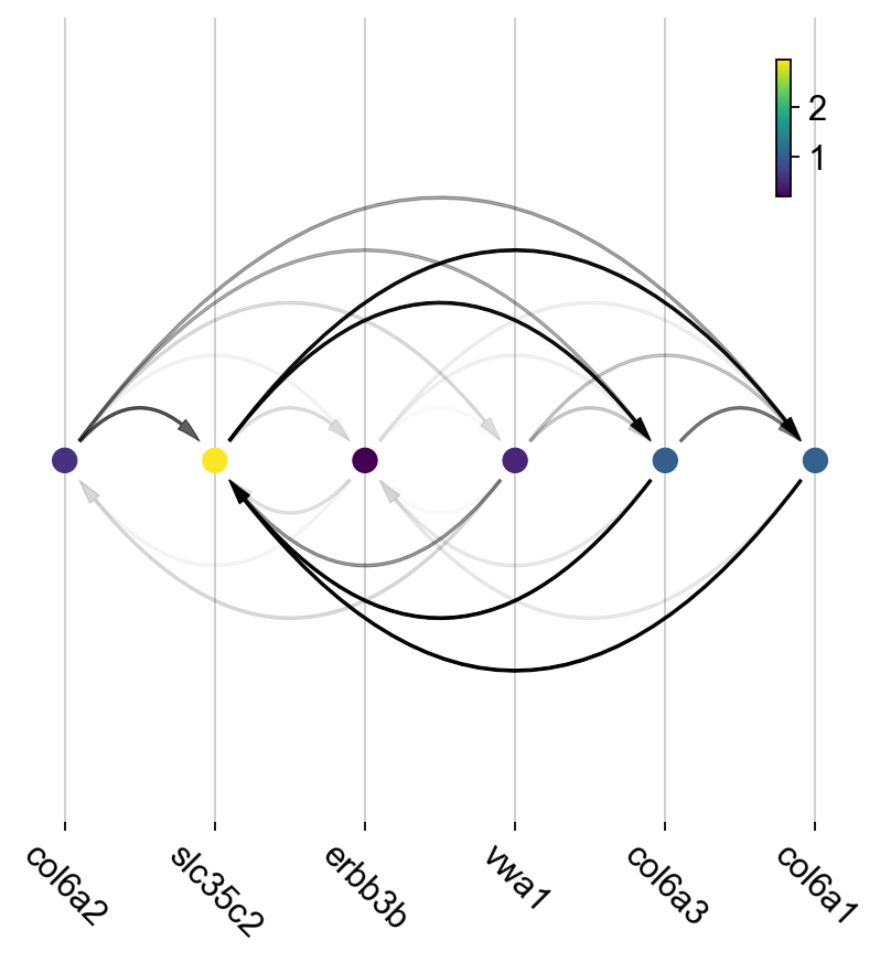
With the full_reg_rank and full_eff_rank calculated, we can now pass a set of genes of interests and use them to build a regulatory network for any specific cell type and then visualize the network with either an arcPlot or a circosPlot, etc.

We build networks for each cell type by passing the argument cluster = "Cell_type" to dynamo.vf.build_network_per_cluster() function. The edges and their weights are based on the above ranking full regulator/effector dictionaries (pass as values to the full_reg_rank and full_eff_rank arguments).

Interesting, Jacobian analysis revealed potential regulation of the chondrocyte marker slc36c2 by the pigment regulator erbb3, consistent with previous reports that EGFR (erbb3) signaling is critical for maintaining the chondrocyte lineage (Fisher et al. 2007). In addition, this analysis revealed a strong connection between chondrocyte-specific markers col6a3, col6a, col6a2, and vwa1.

Here we will use a few key gene in the “unknown” cell cluster to build a regulatory network based on the estimated cell-wise Jacobian matrices of chondrocyte cells.

import networkx as nx
import numpy as np

unknown_cell_type_regulators = ["erbb3b", "col6a3", "vwa1", "slc35c2", "col6a2", "col6a1"]
edges_list = dyn.vf.build_network_per_cluster(adata,
                                              cluster='Cell_type',
                                              cluster_names=None,
                                              full_reg_rank=full_reg_rank,
                                              full_eff_rank=full_eff_rank,
                                              genes=np.unique(unknown_cell_type_regulators),
                                              n_top_genes=100)
network = nx.from_pandas_edgelist(edges_list['Unknown'], 'regulator', 
                                  'target', edge_attr='weight', create_using=nx.DiGraph())

|-----> [iterating reg_groups] in progress: 100.0000%|-----> [iterating reg_groups] completed [1.4136s]

Network can then be visualized as an Arcplot:

ax=dyn.pl.arcPlot(adata, cluster="Cell_type", cluster_name="Unknown", 
                  edges_list=None, network=network, color="M_s")

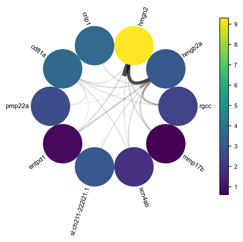
Similarly, network can also be built with other criteria and visualized with other plots, like the circos plot or hive Plot. For example, we can select 10 top genes with highest absolute acceleration values in Unknown cell type.

selected_genes = adata.uns['rank_abs_acceleration']['Unknown'][:10]

edges_list = dyn.vf.build_network_per_cluster(adata,
                                              cluster='Cell_type',
                                              cluster_names=None,
                                              full_reg_rank=full_reg_rank,
                                              full_eff_rank=full_eff_rank,
                                              genes=selected_genes,
                                              n_top_genes=1000)

|-----> [iterating reg_groups] in progress: 100.0000%|-----> [iterating reg_groups] completed [1.6208s]

We can then focus on analyzing Unknown cell type network and construct networkx graph structure for Unknown cell group. We next constrain the edges by removing all edges with weight <= 0.0015.

network = nx.from_pandas_edgelist(edges_list['Unknown'].drop_duplicates().query("weight > 0.0015"), 
                                  'regulator', 'target', 
                                  edge_attr='weight',
                                  create_using=nx.DiGraph())

Before drawing a circos plot, we can insert attributes into networkx Graph object. In the code cell below, we assign average M_s values to each cluster to color the nodes in the circos plot later.

color_key = "M_s"
cluster_key = "Cell_type"
selected_cluster = "Unknown"
adata_layer_key = "M_s"
for node in network.nodes:
    network.nodes[node]["M_s"] = adata[:, node].layers["M_s"].mean()

for edge in network.edges:
    network.edges[edge]["weight"] *= 1000

Lastly, we can visulize the network with dynamo.pl.circosPlot().

dyn.configuration.set_figure_params(background='white')
dyn.pl.circosPlot(network, node_color_key="M_s", 
                  show_colorbar=True, 
                  edge_alpha_scale=0.7, edge_lw_scale=0.7)

<Axes: >

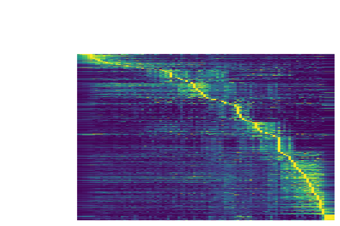
Visualize gene expression, velocity, acceleration, curvature as a function of vector field based pseudotime.

Here we can apply dynamo.ext.ddhodge() to first obtain a measure of pseudotime that is based on learned vector field function. Then we can visualize gene expression, velocity, acceleration, curvature as a function of vector field based pseudotime to reveal different aspects of gene expression kinetics over time.

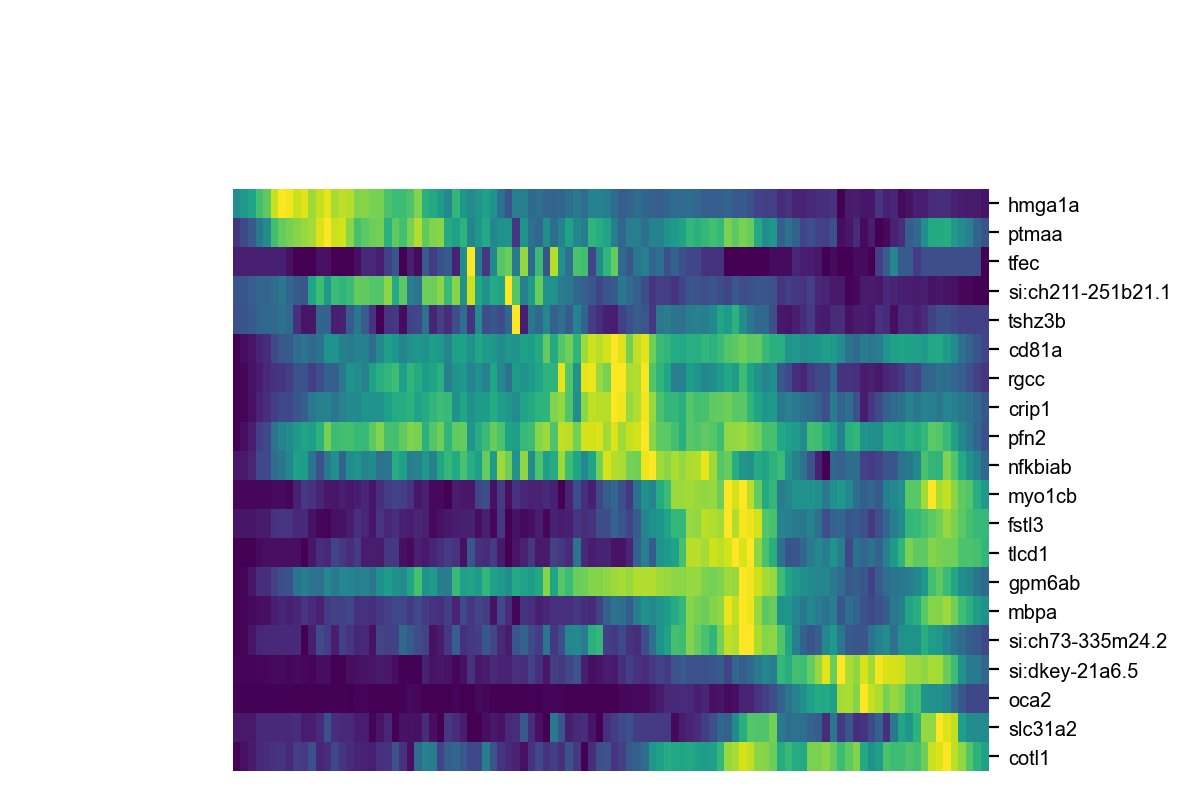
The kinetic heatmap shown below indicates that there are a few distinct stages of gene expression changes (or velocity, acceleration, curvature, etc.) during zebrafish pigmentation.

dyn.ext.ddhodge(adata, basis='pca')

|-----> graphizing vectorfield...
|-----------? nbrs_idx argument is ignored and recomputed because nbrs_idx is not None and return_nbrs=True
|-----------> calculating neighbor indices...
|-----> method arg is None, choosing methods automatically...
|-----------> method ball_tree selected
|-----> [ddhodge completed] completed [25.4098s]

transition_genes = adata.var_names[adata.var.use_for_transition]

Visualize the gene expression dynamics as a function of vector field based pseudotime (x-axis).

dyn.pl.kinetic_heatmap(adata, 
                       genes=transition_genes, 
                       tkey='pca_ddhodge_potential',
                       gene_order_method='maximum', 
                       mode='pseudotime', 
                       color_map='viridis',
                       yticklabels=False,  
                       figsize=(6,4)
                      )

Note that if you want to visualize the gene expression for a specific cell lineage, you can subset the adata via something like (the same applies to other kinetic heatmaps):

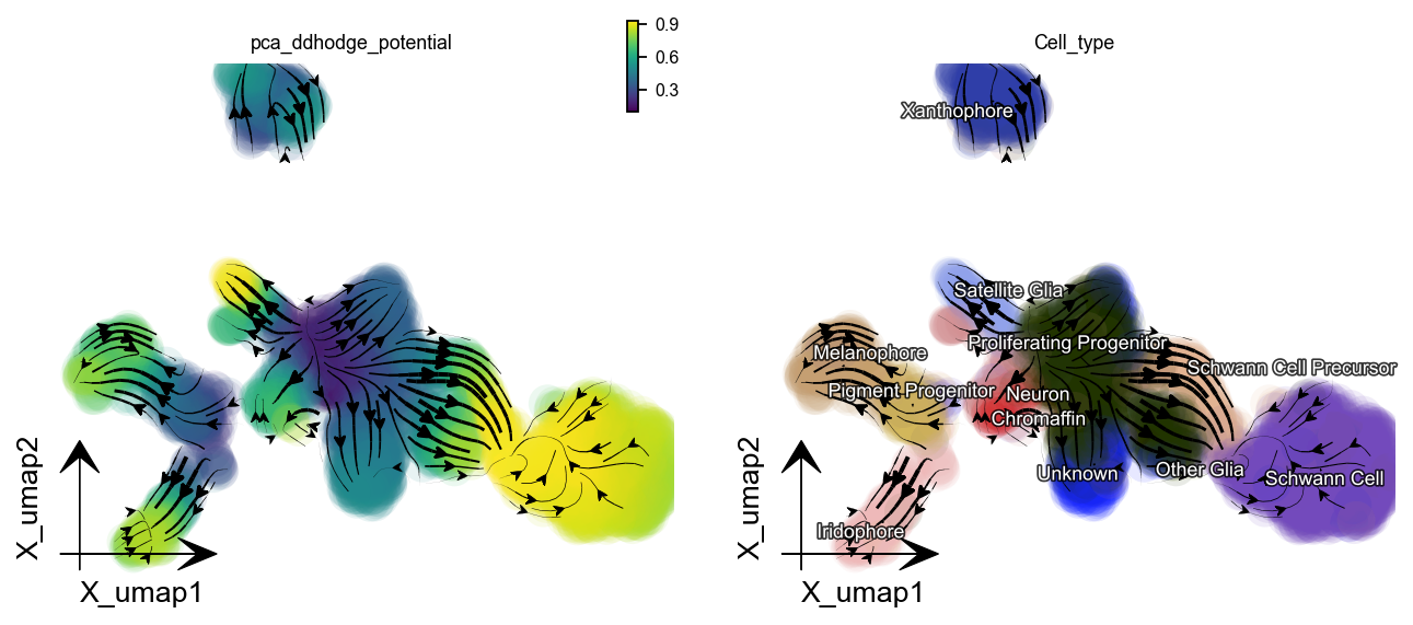
Let us check the melanophore lineage by cross referencing the vector-field based pseudotime and the streamline plots, overlaied with cell-type annotations.

dyn.pl.streamline_plot(adata, color=['pca_ddhodge_potential', 'Cell_type'],
                       figsize=(5,4),s_kwargs_dict={'adjust_legend':True,'dpi':80},)

|-----> method arg is None, choosing methods automatically...
|-----------> method kd_tree selected
|-----------> plotting with basis key=X_umap
|-----------> plotting with basis key=X_umap
|-----------> skip filtering Cell_type by stack threshold when stacking color because it is not a numeric type

We can then collect cells from Proliferating Progenitor, Pigment Progenitor, Melanophore that forms the melanophore lineage by subseting adata object. This adata subset is then used to visualize the expression kinetic heatmap for the melanophore lineage.

subset = adata[adata.obs.Cell_type.isin(['Proliferating Progenitor', 
                                         'Pigment Progenitor', 
                                         'Melanophore'])]

dyn.pl.kinetic_heatmap(subset, 
                       genes=transition_genes[:20], 
                       tkey='pca_ddhodge_potential',
                       gene_order_method='maximum', 
                       mode='pseudotime', 
                       color_map='viridis',
                       yticklabels=True,   
                       figsize=(6,4)
                      )

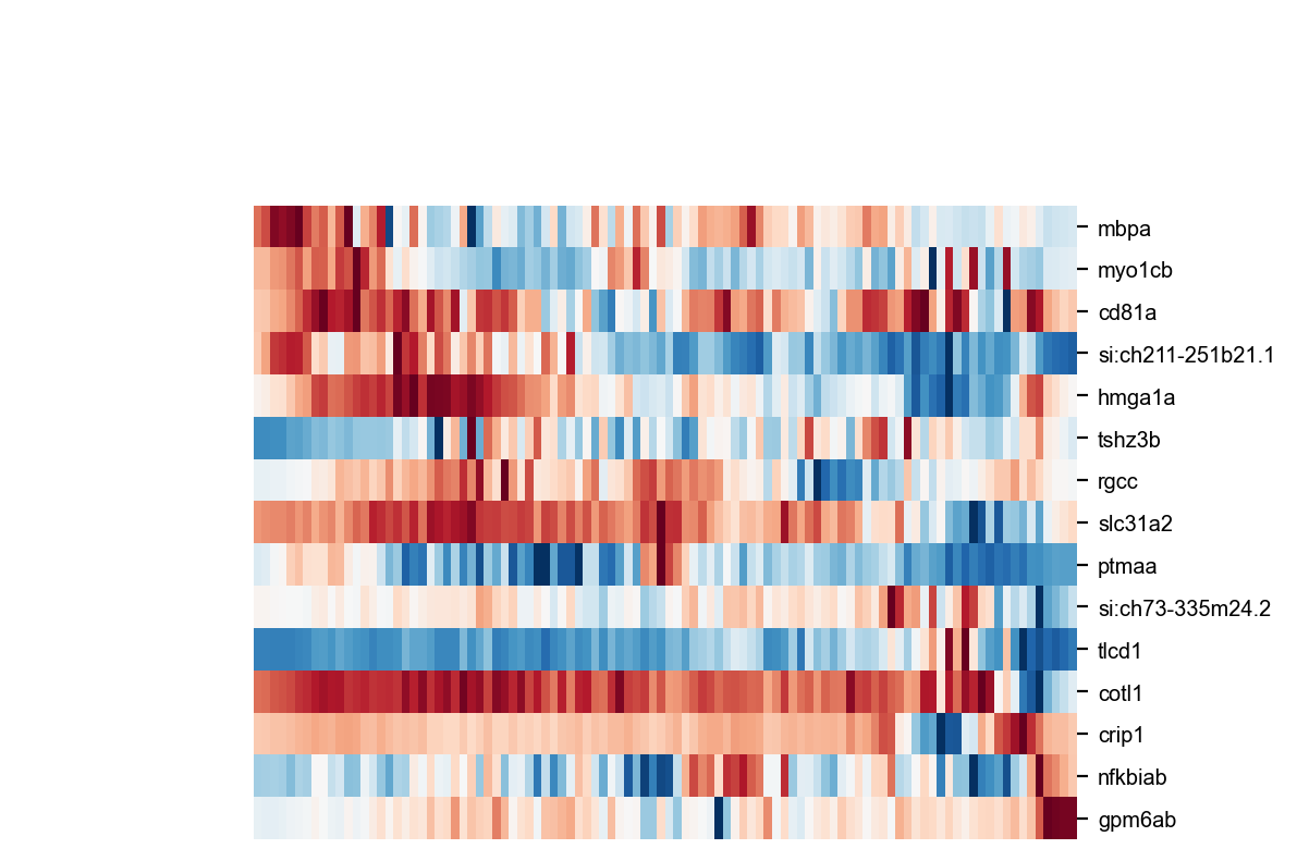
Visualize the gene velocity dynamics as a function of vector field based pseudotime (x-axis).

dyn.pl.kinetic_heatmap(adata, 
                       genes=transition_genes[:20], 
                       tkey='pca_ddhodge_potential',
                       gene_order_method='maximum', 
                       layer='velocity_S',
                       mode='pseudotime', 
                       color_map='RdBu_r',
                       yticklabels=True, 
                       figsize=(6,4)
                      )

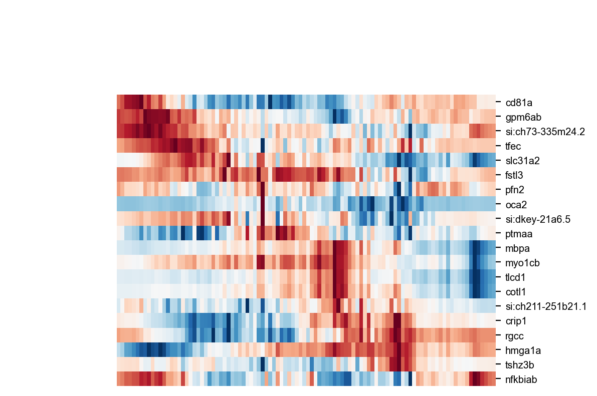
Visualize the gene acceleration dynamics as a function of vector field based pseudotime (x-axis).

dyn.pl.kinetic_heatmap(adata, 
                       genes=transition_genes[:20], 
                       tkey='pca_ddhodge_potential',
                       gene_order_method='maximum', 
                       layer='acceleration',
                       mode='pseudotime', 
                       yticklabels=True,  
                       color_map='RdBu_r',
                      figsize=(6,4))

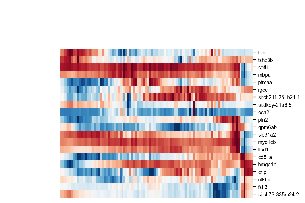
Visualize the gene curvature dynamics as a function of vector field based pseudotime (x-axis).

dyn.pl.kinetic_heatmap(adata, 
                       genes=transition_genes[:20], 
                       tkey='pca_ddhodge_potential',
                       gene_order_method='maximum', 
                       layer='curvature',
                       mode='pseudotime', 
                       yticklabels=True,  
                       color_map='RdBu_r',
                      figsize=(6,4))

Build transition graph between cell states

When projecting high-dimensional RNA velocity vectors into low-dimensional space, dynamo builds a cell-wise transition matrix by translating the velocity vector direction and the spatial relationship of each cell to its neighbors to transition probabilities, similar to velocyto, etc. dynamo uses a few different kernels to build such a transition matrix which can then be used to run Markov chain simulations, as we will demonstrate in future.

On the other hand, it is of great interests to obtain a transition graph between cell types (states). dynamo implements such a functionality with a few methods which effectively creates a model that summarizes the possible cell type transitions based on the reconstructed Markov transition matrix between cell or the vector field function.

To achieve this, we only need to build a state graph with dynamo.pd.state_graph() in a specific basis for a specific grouping. For example, we can use the vector field integration based method vf to build a transition graph between different cell types:

%%capture
dyn.pd.state_graph(adata, group='Cell_type', basis='pca', method='vf')

|-----> Estimating the transition probability between cell types...
|-----> Applying vector field
|-----> [KDTree parameter preparation computation] in progress: 0.0000%|-----> [KDTree computation] completed [0.0017s]
|-----> [iterate groups] in progress: 100.0000%|-----> [iterate groups] completed [94.9211s]
|-----> [State graph estimation] completed [0.0021s]

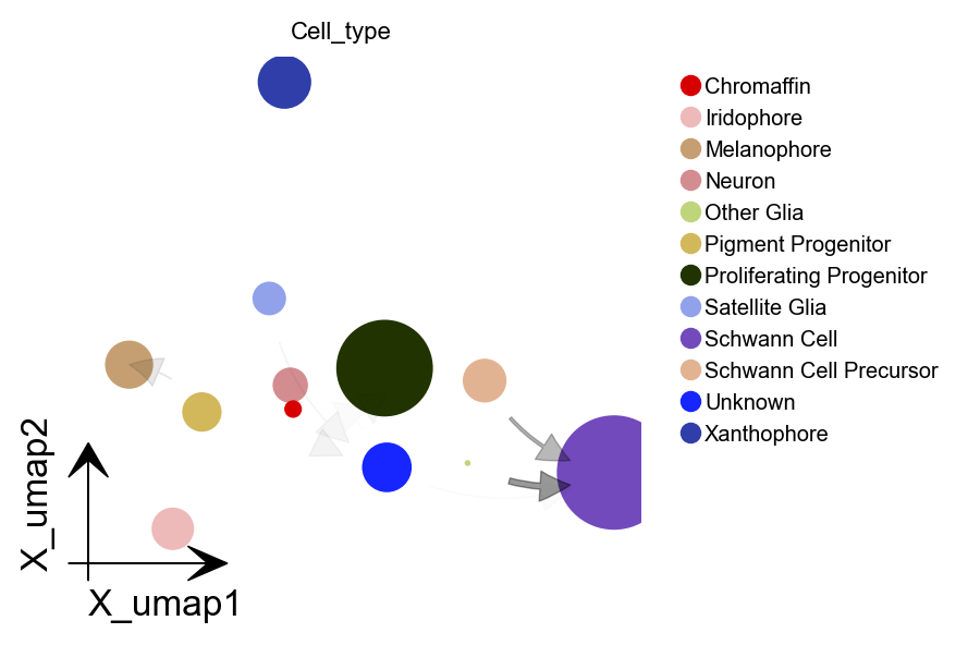
Next, a state graph can be visualized with dynamo.pl.state_graph().

dyn.pl.state_graph(adata, 
                   color=['Cell_type'], 
                   group='Cell_type', 
                   basis='umap', 
                   show_legend='upper right',
                   method='vf',
                  figsize=(4.5,3))

|-----------> plotting with basis key=X_umap
|-----------> skip filtering Cell_type by stack threshold when stacking color because it is not a numeric type

<Figure size 600x400 with 0 Axes>

Save results

save ranking information to an excel file

dynamo provides an utility function to automatically save the ranking related data frames to an excel file with each ranking information saved to a separate sheet in the xlsx file.

dyn.export_rank_xlsx(adata, path="result/rank_info.xlsx")

|-----> saving sheet: rank_velocity_S
|-----> saving sheet: rank_abs_velocity_S
|-----> saving sheet: rank_acceleration
|-----> saving sheet: rank_abs_acceleration
|-----> saving sheet: rank_curvature
|-----> saving sheet: rank_abs_curvature
|-----> saving sheet: rank_div_gene_jacobian_pca

Save data with pickle dumping or pandas dataframe to_csv

In addition, you can directly either export data to a csv file via:

adata.uns['rank_acceleration'].to_csv('./zebrafish_vf_rank_acceleration.csv')

Alternatively, you can save the data via pickle dump:

import pickle

pickle.dump(adata.uns['rank_acceleration'], open('./zebrafish_vf_rank_acceleration.p', 'wb'))
pickle.dump(full_reg_rank, open('./zebrafish_vf_full_reg_rank.p', 'wb'))

_acceleration_rank = pickle.load(open('./zebrafish_vf_rank_acceleration.p', 'rb'))
_acceleration_rank.head(2)

Dynamo save utility

Note that there may be intermediate results stored in adata.uns that can may lead to errors when writing the h5ad object. For now, we suggest users to call dynamo.cleanup()(adata) first to remove these data objects before saving the adata object.

dyn.cleanup(adata);

call AnnData write_h5ad to save the entire adata information.

adata.write_h5ad("result/tutorial_processed_zebrafish_data.h5ad")

You can load in the data later if need:

_adata = dyn.read_h5ad(("result/tutorial_processed_zebrafish_data.h5ad"))