Dynamo without unspliced/spliced matrix
When you don’t have unspliced/spliced RNA but still want to utilize the velocity/vector field and downstream differential geometry analysis, we can use dynamo.tl.pseudotime_velocity() to convert pseudotime to RNA velocity. Essentially this function computes the gradient of pseudotime and use that to calculate a transition graph (a directed weighted graph) between each cell and use that to learn either the velocity on low dimensional embedding as well as the gene-wise RNA velocity.
import warnings
warnings.filterwarnings('ignore')
warnings.filterwarnings("ignore", message="numpy.dtype size changed")
import dynamo as dyn
dyn.configuration.set_figure_params('dynamo', background='white')
dyn.pl.style(font_path='Arial')
dyn.get_all_dependencies_version()
%load_ext autoreload
%autoreload 2
Using already downloaded Arial font from: /tmp/dynamo_arial.ttf
Registered custom font as: Arial
███ ████████
█████ █████ █████ █████ ███ █████
██████ ██████ ██████ ████████ ████
___ ████ ███
| \ _ _ _ _ __ _ _ __ ___ ███
| |) | || | ' \/ _` | ' \/ _ \█████ ███
|___/ \_, |_||_\__,_|_|_|_\___/█████ ████
|__/ ███ █████
Tutorial: https://dynamo-release.readthedocs.io/
█████
| package | umap-learn | typing-extensions | tqdm | statsmodels | setuptools | session-info | seaborn | scipy | requests | pynndescent | pre-commit | pandas | openpyxl | numdifftools | numba | networkx | mudata | matplotlib | loompy | leidenalg | igraph | dynamo-release | colorcet | anndata |
|---|---|---|---|---|---|---|---|---|---|---|---|---|---|---|---|---|---|---|---|---|---|---|---|---|
| version | 0.5.7 | 4.13.2 | 4.67.1 | 0.14.4 | 79.0.0 | 1.0.1 | 0.13.2 | 1.11.4 | 2.32.3 | 0.5.13 | 4.2.0 | 2.2.3 | 3.1.5 | 0.9.41 | 0.60.0 | 3.4.2 | 0.3.1 | 3.10.3 | 3.0.8 | 0.10.2 | 0.11.8 | 1.4.2rc1 | 3.1.0 | 0.11.4 |
Load data
To demonstrate the appproach in this tutorial, we will use a scRNA-seq dataset of human bone marrow Setty et al., 2019, which can be conveniently acessed through bone_marrow.
#adata=dyn.read('data/setty_bone_marrow.h5ad')
adata=dyn.sample_data.bone_marrow()
adata
|-----> Downloading data to ./data/bone_marrow.h5ad
|-----> File ./data/bone_marrow.h5ad already exists.
AnnData object with n_obs × n_vars = 5780 × 27876
obs: 'clusters', 'palantir_pseudotime', 'palantir_diff_potential'
var: 'palantir'
uns: 'clusters_colors', 'palantir_branch_probs_cell_types'
obsm: 'MAGIC_imputed_data', 'X_tsne', 'palantir_branch_probs'
layers: 'spliced', 'unspliced'
Since we use pre-computed dimensionality reduction information, this tutorial is for demonstration purposes only. Therefore, we directly assign X_tsne to X_umap.
adata.obsm['X_umap']=adata.obsm['X_tsne']
Preprocess
We use the same data preprocessing method as in the Zebrafish pigmentation tutorial. Specific parameter definitions can be found in the original tutorial.
preprocessor = dyn.pp.Preprocessor(cell_cycle_score_enable=True)
preprocessor.preprocess_adata(adata, recipe='monocle')
|-----> Running monocle preprocessing pipeline...
|-----------> filtered out 0 outlier cells
|-----------> filtered out 20894 outlier genes
|-----> PCA dimension reduction
|-----> <insert> X_pca to obsm in AnnData Object.
|-----> computing cell phase...
|-----> [Cell Phase Estimation] completed [92.7317s]
|-----> [Cell Cycle Scores Estimation] completed [1.1006s]
|-----> [Preprocessor-monocle] completed [11.8188s]
dyn.tl.reduceDimension(adata)
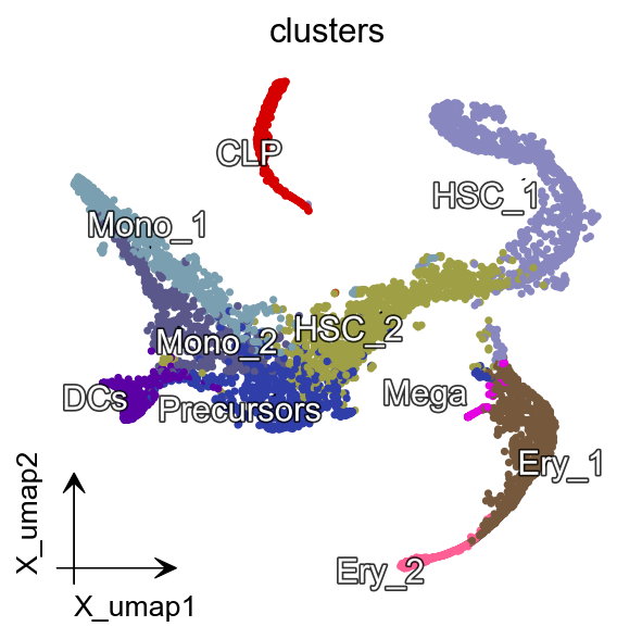
dyn.pl.umap(adata, color='clusters',
figsize=(4,4),pointsize=0.05,alpha=1,
adjust_legend=True,arrow_scale=8)
|-----> retrieve data for non-linear dimension reduction...
|-----? adata already have basis umap. dimension reduction umap will be skipped!
set enforce=True to re-performing dimension reduction.
|-----> Start computing neighbor graph...
|-----------> X_data is None, fetching or recomputing...
|-----> fetching X data from layer:None, basis:pca
|-----> method arg is None, choosing methods automatically...
|-----------> method pynn selected
|-----> [UMAP] completed [35.9859s]
|-----------> plotting with basis key=X_umap
|-----------> skip filtering clusters by stack threshold when stacking color because it is not a numeric type
Convert pseudotime to RNA velocity
Essentially this function computes the gradient of pseudotime and use that to calculate a transition graph (a directed weighted graph) between each cell and use that to learn either the velocity on low dimensional embedding as well as the gene-wise RNA velocity.
We use the expression matrix X to replace the splicing matrix M_s.
adata.layers['M_s']=adata.X
dyn.tl.pseudotime_velocity(adata,
pseudotime='palantir_pseudotime')
|-----> Embrace RNA velocity and velocity vector field analysis for pseudotime...
|-----> Retrieve neighbor graph and pseudotime...
|-----> Computing transition graph via calculating pseudotime gradient with hodge method...
|-----> Use pseudotime transition matrix to learn low dimensional velocity projection.
|-----> [projecting velocity vector to low dimensional embedding] in progress: 100.0000%|-----> [projecting velocity vector to low dimensional embedding] completed [1.6000s]
|-----> Use pseudotime transition matrix to learn gene-wise velocity vectors.
|-----> [projecting velocity vector to low dimensional embedding] in progress: 100.0000%|-----> [projecting velocity vector to low dimensional embedding] completed [41.5870s]
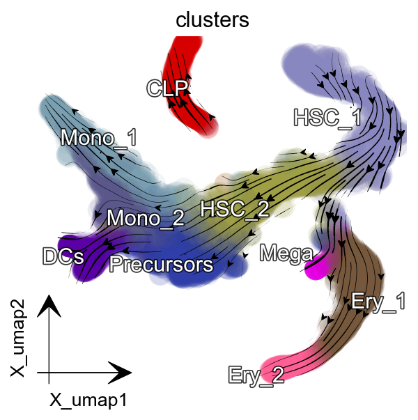
Visualization
All visualization functions and tutorials are consistent with the Zebrafish pigmentation tutorial.
dyn.pl.streamline_plot(adata, color=['clusters'],
basis='umap', show_legend='on data',
s_kwargs_dict={'adjust_legend':True},
show_arrowed_spines=False,
figsize=(4,4),arrow_scale=8)
|-----> method arg is None, choosing methods automatically...
|-----------> method kd_tree selected
|-----------> plotting with basis key=X_umap
|-----------> skip filtering clusters by stack threshold when stacking color because it is not a numeric type
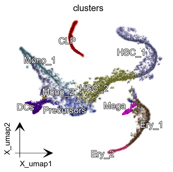
dyn.pl.cell_wise_vectors(adata, color=['clusters'], basis='umap',
show_legend='on data', quiver_length=6,
quiver_size=6, pointsize=0.1,
s_kwargs_dict={'adjust_legend':True},
show_arrowed_spines=False,
figsize=(4,4),arrow_scale=8)
|-----> X shape: (5780, 2) V shape: (5780, 2)
|-----------> plotting with basis key=X_umap
|-----------> skip filtering clusters by stack threshold when stacking color because it is not a numeric type
# you can set `verbose = 1/2/3` to obtain different levels of running information of vector field reconstruction
dyn.vf.VectorField(adata, basis='umap',pot_curl_div=True)
|-----> VectorField reconstruction begins...
|-----> Retrieve X and V based on basis: UMAP.
Vector field will be learned in the UMAP space.
|-----> Generating high dimensional grids and convert into a row matrix.
|-----> Learning vector field with method: sparsevfc.
|-----> [SparseVFC] begins...
|-----> Sampling control points based on data velocity magnitude...
|-----> method arg is None, choosing methods automatically...
|-----------> method kd_tree selected
|-----> [SparseVFC] completed [5.0012s]
|-----> Running ddhodge to estimate vector field based pseudotime in umap basis...
|-----> graphizing vectorfield...
|-----------> calculating neighbor indices...
|-----> method arg is None, choosing methods automatically...
|-----------> method kd_tree selected
|-----------> not all cells are used, set diag to 1...
|-----------> Constructing W matrix according upsampling=True and downsampling=True options...
|-----> [ddhodge completed] completed [25.6764s]
|-----> Computing curl...
|-----> Computing divergence...
|-----> [VectorField] completed [31.6486s]
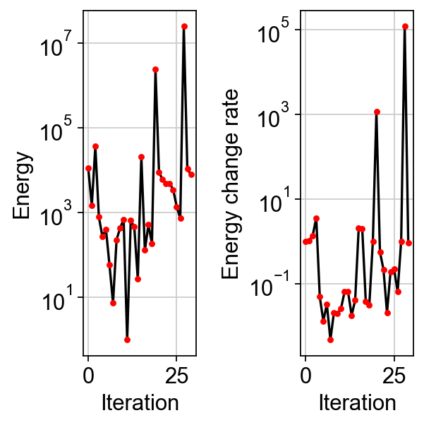
dyn.pl.plot_energy(adata, basis='umap')
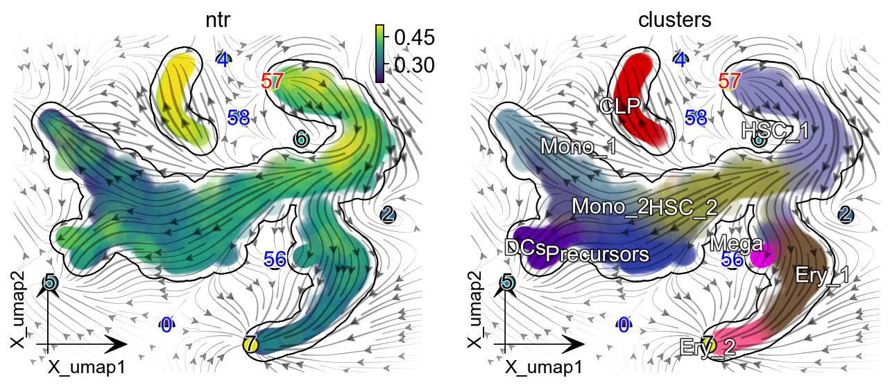
dyn.pl.topography(
adata, basis='umap', background='white',
color=['ntr', 'clusters'],
streamline_color='black',
s_kwargs_dict={'adjust_legend':True,'dpi':80},
show_legend='on data', frontier=True,
figsize=(5,4),markersize=100,s=100,
)
|-----> Vector field for umap is but its topography is not mapped. Mapping topography now ...
|-----> method arg is None, choosing methods automatically...
|-----------> method kd_tree selected
|-----------> plotting with basis key=X_umap
|-----------> plotting with basis key=X_umap
|-----------> skip filtering clusters by stack threshold when stacking color because it is not a numeric type
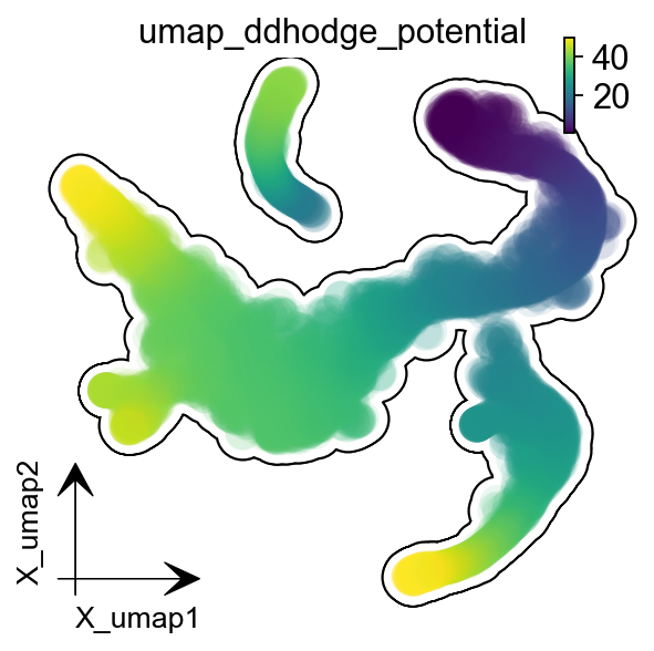
dyn.pl.umap(adata, color='umap_ddhodge_potential',
frontier=True,figsize=(4,4))
|-----------> plotting with basis key=X_umap
progenitor = adata.obs_names[adata.obs.clusters.isin(['HSC_1'])]
len(progenitor)
1118
dyn.pd.fate(adata, basis='umap', init_cells=progenitor,
interpolation_num=100, direction='forward',
inverse_transform=False, average=False, cores=10)
AnnData object with n_obs × n_vars = 5780 × 27876
obs: 'clusters', 'palantir_pseudotime', 'palantir_diff_potential', 'nGenes', 'nCounts', 'pMito', 'pass_basic_filter', 'spliced_Size_Factor', 'initial_spliced_cell_size', 'unspliced_Size_Factor', 'initial_unspliced_cell_size', 'Size_Factor', 'initial_cell_size', 'ntr', 'cell_cycle_phase', 'control_point_umap', 'inlier_prob_umap', 'obs_vf_angle_umap', 'umap_ddhodge_sampled', 'umap_ddhodge_div', 'umap_potential', 'umap_ddhodge_potential', 'curl_umap', 'divergence_umap'
var: 'palantir', 'nCells', 'nCounts', 'pass_basic_filter', 'log_cv', 'log_m', 'score', 'frac', 'use_for_pca', 'ntr'
uns: 'clusters_colors', 'palantir_branch_probs_cell_types', 'pp', 'velocyto_SVR', 'feature_selection', 'PCs', 'explained_variance_ratio_', 'pca_mean', 'cell_phase_order', 'cell_phase_genes', 'neighbors', 'VecFld_umap', 'fate_umap'
obsm: 'MAGIC_imputed_data', 'X_tsne', 'palantir_branch_probs', 'X_umap', 'X_pca', 'cell_cycle_scores', 'velocity_umap', 'velocity_umap_SparseVFC', 'X_umap_SparseVFC'
layers: 'spliced', 'unspliced', 'X_spliced', 'X_unspliced', 'M_s', 'velocity_S'
obsp: 'distances', 'connectivities', 'pseudotime_transition_matrix'
%matplotlib inline
import matplotlib.pyplot as plt
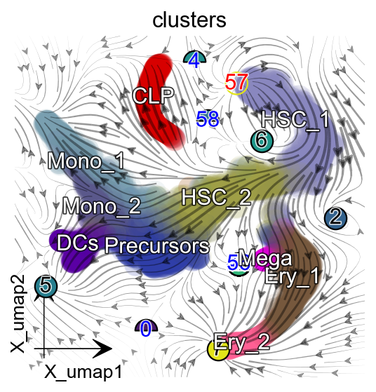
fig, ax = plt.subplots(figsize=(4,4))
ax = dyn.pl.topography(adata, color='clusters',
ax=ax, save_show_or_return='return',
arrow_scale=10)
|-----> Vector field for umap is but its topography is not mapped. Mapping topography now ...
|-----> method arg is None, choosing methods automatically...
|-----------> method kd_tree selected
|-----------> plotting with basis key=X_umap
|-----------> skip filtering clusters by stack threshold when stacking color because it is not a numeric type
%matplotlib inline
instance = dyn.mv.StreamFuncAnim(adata=adata, color='clusters', ax=ax)
|-----? the number of cell states with fate prediction is more than 50. You may want to lower the max number of cell states to draw via cell_states argument.
|-----------> plotting with basis key=X_umap
|-----------> skip filtering clusters by stack threshold when stacking color because it is not a numeric type
%matplotlib notebook
import matplotlib
matplotlib.rcParams['animation.embed_limit'] = 2**64 # Ensure all frames will be embedded.
from matplotlib import animation
import numpy as np
anim = animation.FuncAnimation(instance.fig,
instance.update,
init_func=instance.init_background,
frames=np.arange(100),
interval=100, blit=True)
plt.show()
from IPython.display import HTML
HTML(anim.to_jshtml()) # 或 HTML(anim.to_html5_video())
adata.uns['clusters_colors']
{'Ery_1': '#76583d',
'HSC_1': '#8987bf',
'Mono_1': '#799fb0',
'Precursors': '#2f3ea8',
'Mega': '#e400e3',
'HSC_2': '#9f9f46',
'Mono_2': '#5a588b',
'Ery_2': '#ff5f94',
'DCs': '#5a00a4',
'CLP': '#d70000'}
dyn.configuration.set_figure_params('dynamo', background='black')
X_grid, V_grid=dyn.pl.compute_velocity_on_grid(
adata.obsm['X_umap'],
adata.obsm['velocity_umap']
)
# Full usage with scanpy data and custom parameters
animation = dyn.pl.animate_streamplot(
X_grid, V_grid, adata,
color='clusters', palette=adata.uns['clusters_colors'],
n_frames=50, alpha_animate=0.8,
saveto='result/streamlineplot_pancrea.gif'
)
from IPython.core.display import display, HTML
HTML(animation.to_jshtml()) # embedding to jupyter notebook.