scEU-seq: organoid kinetic analysis
This tutorial demonstrates single-cell kinetic analysis of intestine organoid data using dynamo with scEU-seq technology. We analyze the intestine organoid data from Battich, et al (2020), showing how dynamo can be used to perform kinetic analysis on scEU-seq datasets. This is the second tutorial in our scEU-seq series - please refer to the cell cycle tutorial for details on analyzing cell cycle datasets.
import warnings
warnings.filterwarnings('ignore')
warnings.filterwarnings("ignore", message="numpy.dtype size changed")

import dynamo as dyn

dyn.configuration.set_figure_params('dynamo', background='white')
dyn.pl.style(font_path='Arial')
dyn.get_all_dependencies_version()

%load_ext autoreload
%autoreload 2
Using already downloaded Arial font from: /tmp/dynamo_arial.ttf
Registered custom font as: Arial


 ███                               ████████
█████   █████    █████    █████    ███   █████
   ██████   ██████   ██████   ████████      ████
  ___                           ████            ███
 |   \ _  _ _ _  __ _ _ __  ___                 ███
 | |) | || | ' \/ _` | '  \/ _ \█████           ███
 |___/ \_, |_||_\__,_|_|_|_\___/█████       ████
       |__/                        ███   █████
Tutorial: https://dynamo-release.readthedocs.io/
                                     █████
| package | umap-learn | typing-extensions | tqdm | statsmodels | setuptools | session-info | seaborn | scipy | requests | pynndescent | pre-commit | pandas | openpyxl | numdifftools | numba | networkx | mudata | matplotlib | loompy | leidenalg | igraph | dynamo-release | colorcet | anndata |
|---|---|---|---|---|---|---|---|---|---|---|---|---|---|---|---|---|---|---|---|---|---|---|---|---|
| version | 0.5.7 | 4.13.2 | 4.67.1 | 0.14.4 | 79.0.0 | 1.0.1 | 0.13.2 | 1.11.4 | 2.32.3 | 0.5.13 | 4.2.0 | 2.2.3 | 3.1.5 | 0.9.41 | 0.60.0 | 3.4.2 | 0.3.1 | 3.10.3 | 3.0.8 | 0.10.2 | 0.11.8 | 1.4.2rc1 | 3.1.0 | 0.11.4 |
Load data
We load the scEU-seq organoid dataset using dynamo.sample_data.scEU_seq_organoid().
organoid = dyn.sample_data.scEU_seq_organoid()
|-----> Downloading scEU_seq data
|-----> Downloading data to ./data/organoid.h5ad
|-----> in progress: 99.0108%|-----> [download] completed [72.9405s]
organoid
AnnData object with n_obs × n_vars = 3831 × 9157
    obs: 'well_id', 'batch_id', 'treatment_id', 'log10_gfp', 'rotated_umap1', 'rotated_umap2', 'som_cluster_id', 'monocle_branch_id', 'monocle_pseudotime', 'exp_type', 'time'
    var: 'ID', 'NAME'
    layers: 'sl', 'su', 'ul', 'uu'
# mapping:
cell_mapper = {
    '1': 'Enterocytes',
    '2': 'Enterocytes',
    '3': 'Enteroendocrine',
    '4': 'Enteroendocrine progenitor',
    '5': 'Tuft cells',
    '6': 'TA cells',
    '7': 'TA cells',
    '8': 'Stem cells',
    '9': 'Paneth cells',
    '10': 'Goblet cells',
    '11': 'Stem cells',
 }

organoid.obs['cell_type'] = organoid.obs.som_cluster_id.map(cell_mapper).astype('str')
Typical dynamo analysis workflow
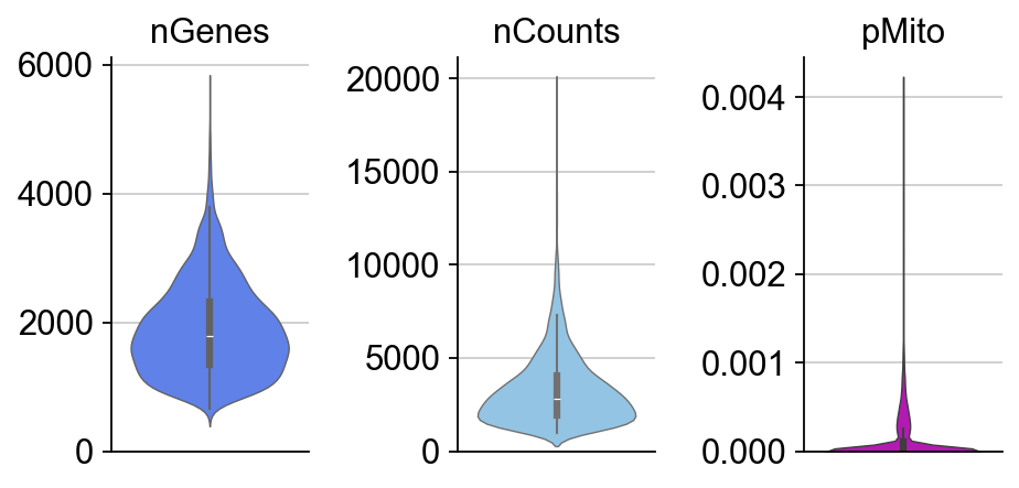
We perform the standard preprocessing and analysis steps using dynamo’s comprehensive workflow.
dyn.pl.basic_stats(organoid,figsize=(2,3))
organoid
AnnData object with n_obs × n_vars = 3831 × 9157
    obs: 'well_id', 'batch_id', 'treatment_id', 'log10_gfp', 'rotated_umap1', 'rotated_umap2', 'som_cluster_id', 'monocle_branch_id', 'monocle_pseudotime', 'exp_type', 'time', 'cell_type', 'nGenes', 'nCounts', 'pMito'
    var: 'ID', 'NAME', 'nCells', 'nCounts'
    layers: 'sl', 'su', 'ul', 'uu'
organoid.obs.head()
| well_id | batch_id | treatment_id | log10_gfp | rotated_umap1 | rotated_umap2 | som_cluster_id | monocle_branch_id | monocle_pseudotime | exp_type | time | cell_type | nGenes | nCounts | pMito | |
|---|---|---|---|---|---|---|---|---|---|---|---|---|---|---|---|
| 1 | 14 | 01 | Pulse_120 | 12.8929281522 | 23.0662174225 | -3.47039175034 | 6 | 2 | 6.08688834859 | Pulse | 120 | TA cells | 1054 | 1426.0 | 0.0 |
| 2 | 15 | 01 | Pulse_120 | 5.85486775252 | 25.710735321 | -1.31835341454 | 2 | 2 | 9.14740876358 | Pulse | 120 | Enterocytes | 1900 | 3712.0 | 0.0 |
| 3 | 16 | 01 | Pulse_120 | 7.45690471634 | 26.7709560394 | -1.06682777405 | 2 | 2 | 9.69134627386 | Pulse | 120 | Enterocytes | 2547 | 6969.0 | 0.0 |
| 4 | 17 | 01 | Pulse_120 | 94.2814535609 | 21.2927913666 | 0.0159659013152 | 11 | 2 | 4.2635104705 | Pulse | 120 | Stem cells | 1004 | 1263.0 | 0.0 |
| 5 | 21 | 01 | Pulse_120 | 47.1412266395 | 19.9096126556 | 0.884054124355 | 11 | 1 | 2.62248093423 | Pulse | 120 | Stem cells | 927 | 1144.0 | 0.0 |
organoid.obs.groupby(['exp_type', 'time']).agg('count')
| well_id | batch_id | treatment_id | log10_gfp | rotated_umap1 | rotated_umap2 | som_cluster_id | monocle_branch_id | monocle_pseudotime | cell_type | nGenes | nCounts | pMito | ||
|---|---|---|---|---|---|---|---|---|---|---|---|---|---|---|
| exp_type | time | |||||||||||||
| Chase | 0 | 660 | 660 | 660 | 660 | 660 | 660 | 660 | 660 | 660 | 660 | 660 | 660 | 660 |
| 45 | 821 | 821 | 821 | 821 | 821 | 821 | 821 | 821 | 821 | 821 | 821 | 821 | 821 | |
| 120 | 0 | 0 | 0 | 0 | 0 | 0 | 0 | 0 | 0 | 0 | 0 | 0 | 0 | |
| 360 | 646 | 646 | 646 | 646 | 646 | 646 | 646 | 646 | 646 | 646 | 646 | 646 | 646 | |
| dmso | 0 | 0 | 0 | 0 | 0 | 0 | 0 | 0 | 0 | 0 | 0 | 0 | 0 | |
| Pulse | 0 | 0 | 0 | 0 | 0 | 0 | 0 | 0 | 0 | 0 | 0 | 0 | 0 | 0 |
| 45 | 0 | 0 | 0 | 0 | 0 | 0 | 0 | 0 | 0 | 0 | 0 | 0 | 0 | |
| 120 | 1373 | 1373 | 1373 | 1373 | 1373 | 1373 | 1373 | 1373 | 1373 | 1373 | 1373 | 1373 | 1373 | |
| 360 | 0 | 0 | 0 | 0 | 0 | 0 | 0 | 0 | 0 | 0 | 0 | 0 | 0 | |
| dmso | 331 | 331 | 331 | 331 | 331 | 331 | 331 | 331 | 331 | 331 | 331 | 331 | 331 |
adata = organoid.copy()
adata.obs.time = adata.obs.time.astype('str')
adata.obs.loc[adata.obs['time'] == 'dmso', 'time'] = -1
adata.obs['time'] = adata.obs['time'].astype(float)
adata = adata[adata.obs.time != -1, :]
adata = adata[adata.obs.exp_type == 'Pulse', :]
adata.layers['new'], adata.layers['total'] = adata.layers['ul'] + adata.layers['sl'], adata.layers['su'] + adata.layers['sl'] + adata.layers['uu'] + adata.layers['ul']
del adata.layers['uu'], adata.layers['ul'], adata.layers['su'], adata.layers['sl']
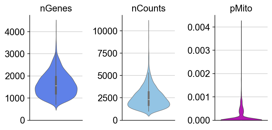
dyn.pp.recipe_monocle(adata, n_top_genes=1000, total_layers=False)
# preprocessor = dyn.pp.Preprocessor(cell_cycle_score_enable=True)
# preprocessor.config_monocle_recipe(adata, n_top_genes=1000)
# preprocessor.preprocess_adata_monocle(adata)
dyn.pl.basic_stats(adata,figsize=(2,3))
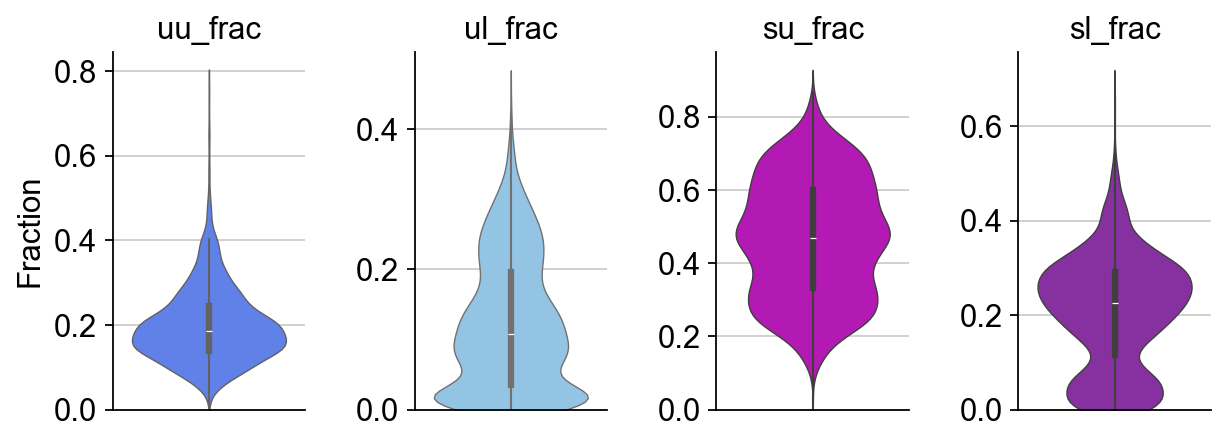
dyn.pl.show_fraction(organoid,figsize=(2,3))
|-----? dynamo.preprocessing.deprecated is deprecated.
|-----> recipe_monocle_keep_filtered_cells_key is None. Using default value from DynamoAdataConfig: recipe_monocle_keep_filtered_cells_key=True
|-----> recipe_monocle_keep_filtered_genes_key is None. Using default value from DynamoAdataConfig: recipe_monocle_keep_filtered_genes_key=True
|-----> recipe_monocle_keep_raw_layers_key is None. Using default value from DynamoAdataConfig: recipe_monocle_keep_raw_layers_key=True
|-----> apply Monocole recipe to adata...
|-----> ensure all cell and variable names unique.
|-----> ensure all data in different layers in csr sparse matrix format.
|-----> ensure all labeling data properly collapased
|-----?
When analyzing labeling based scRNA-seq without providing `tkey`, dynamo will try to use
 `time` as the key for labeling time. Please correct this via supplying the correct `tkey`
if needed.
|-----> detected experiment type: one-shot
|-----? Looks like you are using minutes as the time unit. For the purpose of numeric stability, we recommend using hour as the time unit.
|-----> filtering cells...
|-----> 1373 cells passed basic filters.
|-----> filtering gene...
|-----> 8342 genes passed basic filters.
|-----> calculating size factor...
|-----> selecting genes in layer: X, sort method: SVR...
|-----> size factor normalizing the data, followed by log1p transformation.
|-----> Set <adata.X> to normalized data
|-----> applying PCA ...
|-----> <insert> X_pca to obsm in AnnData Object.
|-----> cell cycle scoring...
|-----> computing cell phase...
|-----> [Cell Phase Estimation] completed [232.9096s]
|-----> [Cell Cycle Scores Estimation] completed [0.1440s]
|-----> [recipe_monocle preprocess] completed [2.9687s]
adata.obs.time = adata.obs.time/60
adata.obs.time  = adata.obs.time.astype('float')
dyn.tl.dynamics(adata, model='deterministic', tkey='time', assumption_mRNA='ss')
dyn.tl.reduceDimension(adata)
|-----> dynamics_del_2nd_moments_key is None. Using default value from DynamoAdataConfig: dynamics_del_2nd_moments_key=False
|-----------> removing existing M layers:[]...
|-----------> making adata smooth...
|-----> calculating first/second moments...
|-----> [moments calculation] completed [13.7746s]
|-----? Your adata only has labeling data, but `NTR_vel` is set to be `False`. Dynamo will reset it to `True` to enable this analysis.
|-----> retrieve data for non-linear dimension reduction...
|-----> [UMAP] using X_pca with n_pca_components = 30
|-----> <insert> X_umap to obsm in AnnData Object.
|-----> [UMAP] completed [10.1453s]
dyn.tl.cell_velocities(adata, ekey='M_t', vkey='velocity_T', enforce=True)
|-----> incomplete neighbor graph info detected: connectivities and distances do not exist in adata.obsp, indices not in adata.uns.neighbors.
|-----> Neighbor graph is broken, recomputing....
|-----> Start computing neighbor graph...
|-----------> X_data is None, fetching or recomputing...
|-----> fetching X data from layer:None, basis:pca
|-----> method arg is None, choosing methods automatically...
|-----------> method ball_tree selected
|-----> [calculating transition matrix via pearson kernel with sqrt transform.] in progress: 100.0000%|-----> [calculating transition matrix via pearson kernel with sqrt transform.] completed [3.9081s]
|-----> [projecting velocity vector to low dimensional embedding] in progress: 100.0000%|-----> [projecting velocity vector to low dimensional embedding] completed [0.4533s]
|-----> method arg is None, choosing methods automatically...
|-----------> method kd_tree selected
AnnData object with n_obs × n_vars = 1373 × 9157
    obs: 'well_id', 'batch_id', 'treatment_id', 'log10_gfp', 'rotated_umap1', 'rotated_umap2', 'som_cluster_id', 'monocle_branch_id', 'monocle_pseudotime', 'exp_type', 'time', 'cell_type', 'nGenes', 'nCounts', 'pMito', 'pass_basic_filter', 'total_Size_Factor', 'initial_total_cell_size', 'Size_Factor', 'initial_cell_size', 'new_Size_Factor', 'initial_new_cell_size', 'ntr', 'cell_cycle_phase'
    var: 'ID', 'NAME', 'nCells', 'nCounts', 'pass_basic_filter', 'score', 'log_cv', 'log_m', 'frac', 'use_for_pca', 'ntr', 'use_for_dynamics', 'use_for_transition'
    uns: 'pp', 'velocyto_SVR', 'PCs', 'explained_variance_ratio_', 'pca_mean', 'pca_fit', 'feature_selection', 'cell_phase_order', 'cell_phase_genes', 'vel_params_names', 'dynamics', 'neighbors', 'umap_fit', 'grid_velocity_umap'
    obsm: 'X_pca', 'X', 'cell_cycle_scores', 'X_umap', 'velocity_umap'
    varm: 'alpha', 'vel_params'
    layers: 'new', 'total', 'X_total', 'X_new', 'M_t', 'M_tt', 'M_n', 'M_tn', 'M_nn', 'velocity_N', 'velocity_T'
    obsp: 'moments_con', 'distances', 'connectivities', 'pearson_transition_matrix'
adata.obsm['X_umap_ori'] = adata.obs.loc[:, ['rotated_umap1', 'rotated_umap2']].values.astype(float)
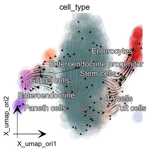
Visualize time-resolved vector flow learned with dynamo
We use dynamo.pl.streamline_plot() to visualize the learned vector field and cellular dynamics.
dyn.tl.cell_velocities(adata, basis='umap_ori')

dyn.pl.streamline_plot(adata, color='cell_type',
                       basis='umap_ori',figsize=(4,4),
                       s_kwargs_dict={'adjust_legend':True},
                      )
Using existing pearson_transition_matrix found in .obsp.
|-----> [projecting velocity vector to low dimensional embedding] in progress: 100.0000%|-----> [projecting velocity vector to low dimensional embedding] completed [0.4446s]
|-----> method arg is None, choosing methods automatically...
|-----------> method kd_tree selected
|-----> method arg is None, choosing methods automatically...
|-----------> method kd_tree selected
|-----------> plotting with basis key=X_umap_ori
|-----------> skip filtering cell_type by stack threshold when stacking color because it is not a numeric type
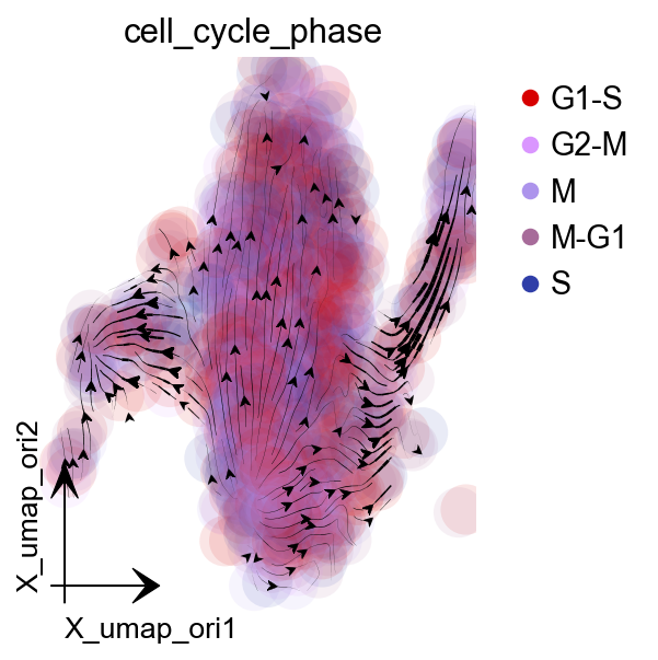
dyn.pl.streamline_plot(adata, color='cell_cycle_phase',
                       basis='umap_ori',figsize=(4,4),
                       show_legend='upper right',
                       s_kwargs_dict={'adjust_legend':True},
)
|-----> method arg is None, choosing methods automatically...
|-----------> method kd_tree selected
|-----------> plotting with basis key=X_umap_ori
|-----------> skip filtering cell_cycle_phase by stack threshold when stacking color because it is not a numeric type
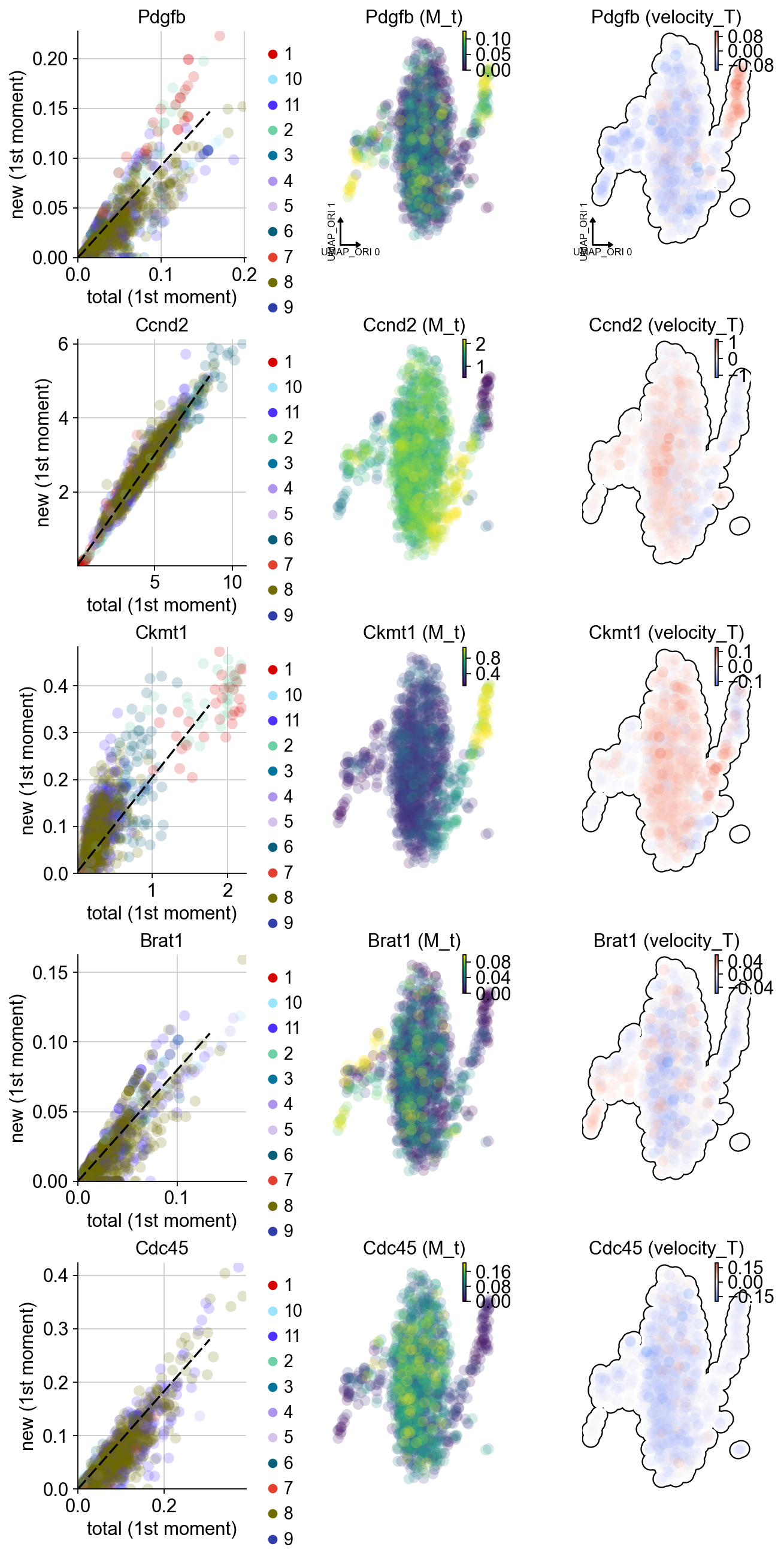
adata.var_names[adata.var.use_for_transition][:5]
Index(['Cdc45', 'Brat1', 'Ccnd2', 'Ckmt1', 'Pdgfb'], dtype='object')
dyn.pl.phase_portraits(adata, genes=['Cdc45', 'Brat1', 'Ccnd2', 'Ckmt1', 'Pdgfb'],
                       color='som_cluster_id', basis='umap_ori',figsize=(3,4))
Animate intestine organoid differentiation
We use dynamo.pd.fate() and dynamo.mv animation capabilities to visualize organoid differentiation dynamics over time.
dyn.vf.VectorField(adata, basis='umap_ori')
|-----> VectorField reconstruction begins...
|-----> Retrieve X and V based on basis: UMAP_ORI.
        Vector field will be learned in the UMAP_ORI space.
|-----> Generating high dimensional grids and convert into a row matrix.
|-----> Learning vector field with method: sparsevfc.
|-----> [SparseVFC] begins...
|-----> Sampling control points based on data velocity magnitude...
|-----> method arg is None, choosing methods automatically...
|-----------> method kd_tree selected
|-----> [SparseVFC] completed [1.1309s]
|-----------> current cosine correlation between input velocities and learned velocities is less than 0.6. Make a 1-th vector field reconstruction trial.
|-----> [SparseVFC] begins...
|-----> Sampling control points based on data velocity magnitude...
|-----> [SparseVFC] completed [1.4815s]
|-----------> current cosine correlation between input velocities and learned velocities is less than 0.6. Make a 2-th vector field reconstruction trial.
|-----> [SparseVFC] begins...
|-----> Sampling control points based on data velocity magnitude...
|-----> [SparseVFC] completed [1.5582s]
|-----------> current cosine correlation between input velocities and learned velocities is less than 0.6. Make a 3-th vector field reconstruction trial.
|-----> [SparseVFC] begins...
|-----> Sampling control points based on data velocity magnitude...
|-----> [SparseVFC] completed [1.5784s]
|-----------> current cosine correlation between input velocities and learned velocities is less than 0.6. Make a 4-th vector field reconstruction trial.
|-----> [SparseVFC] begins...
|-----> Sampling control points based on data velocity magnitude...
|-----> [SparseVFC] completed [1.6330s]
|-----------> current cosine correlation between input velocities and learned velocities is less than 0.6. Make a 5-th vector field reconstruction trial.
|-----? Cosine correlation between input velocities and learned velocities is less than 0.6 after 5 trials of vector field reconstruction.
|-----> [VectorField] completed [7.4842s]
progenitor = adata.obs_names[adata.obs.cell_type == 'Stem cells']
len(progenitor)
1146
from matplotlib import animation
info_genes = adata.var_names[adata.var.use_for_transition]
dyn.pd.fate(adata, basis='umap_ori', init_cells=progenitor[:100],
            interpolation_num=100,  direction='forward',
   inverse_transform=False, average=False)
AnnData object with n_obs × n_vars = 1373 × 9157
    obs: 'well_id', 'batch_id', 'treatment_id', 'log10_gfp', 'rotated_umap1', 'rotated_umap2', 'som_cluster_id', 'monocle_branch_id', 'monocle_pseudotime', 'exp_type', 'time', 'cell_type', 'nGenes', 'nCounts', 'pMito', 'pass_basic_filter', 'total_Size_Factor', 'initial_total_cell_size', 'Size_Factor', 'initial_cell_size', 'new_Size_Factor', 'initial_new_cell_size', 'ntr', 'cell_cycle_phase', 'control_point_umap_ori', 'inlier_prob_umap_ori', 'obs_vf_angle_umap_ori'
    var: 'ID', 'NAME', 'nCells', 'nCounts', 'pass_basic_filter', 'score', 'log_cv', 'log_m', 'frac', 'use_for_pca', 'ntr', 'use_for_dynamics', 'use_for_transition'
    uns: 'pp', 'velocyto_SVR', 'PCs', 'explained_variance_ratio_', 'pca_mean', 'pca_fit', 'feature_selection', 'cell_phase_order', 'cell_phase_genes', 'vel_params_names', 'dynamics', 'neighbors', 'umap_fit', 'grid_velocity_umap', 'grid_velocity_umap_ori', 'cell_type_colors', 'cell_cycle_phase_colors', 'VecFld_umap_ori', 'fate_umap_ori'
    obsm: 'X_pca', 'X', 'cell_cycle_scores', 'X_umap', 'velocity_umap', 'X_umap_ori', 'velocity_umap_ori', 'velocity_umap_ori_SparseVFC', 'X_umap_ori_SparseVFC'
    varm: 'alpha', 'vel_params'
    layers: 'new', 'total', 'X_total', 'X_new', 'M_t', 'M_tt', 'M_n', 'M_tn', 'M_nn', 'velocity_N', 'velocity_T'
    obsp: 'moments_con', 'distances', 'connectivities', 'pearson_transition_matrix'
import matplotlib.pyplot as plt
fig, ax = plt.subplots(figsize=(4,4))
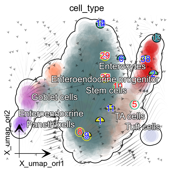
dyn.pl.topography(adata, basis='umap_ori', background='white',
color=['cell_type'], fps_basis='umap_ori',
streamline_color='black', s_kwargs_dict={'adjust_legend':True},
show_legend='on data', frontier=True,ax=ax)
ax.set_aspect(0.8)
|-----------> plotting with basis key=X_umap_ori
|-----------> skip filtering cell_type by stack threshold when stacking color because it is not a numeric type
%%capture
adata.obs['time'] = adata.obs.time.astype('float')
instance = dyn.mv.StreamFuncAnim(adata=adata, basis='umap_ori',
                                 color='cell_type', ax=ax,fig=fig,)
|-----? the number of cell states with fate prediction is more than 50. You may want to lower the max number of cell states to draw via cell_states argument.
import matplotlib
matplotlib.rcParams['animation.embed_limit'] = 2**64 # Ensure all frames will be embedded.

from matplotlib import animation
import numpy as np

anim = animation.FuncAnimation(instance.fig, instance.update, init_func=instance.init_background,
                               frames=np.arange(20), interval=20, blit=True)
from IPython.core.display import display, HTML
HTML(anim.to_jshtml()) # embedding to jupyter notebook.