scEU-seq: cell cycle kinetic analysis

This tutorial demonstrates single-cell kinetic analysis of cell cycle dynamics using dynamo with scEU-seq technology. We analyze the cell cycle dataset from Battich, et al (2020), which represents the first tutorial in our scEU-seq series. For organoid dataset analysis, please refer to the organoid tutorial.

Recently Battich and colleagues reported scEU-seq as a method to sequence mRNA labeled with 5-ethynyl-uridine (EU) in single cells. By developing a very creative labeling strategy (personally this is my favorite labeling strategy from all available labeling based scRNA-seq papers!) they are able to estimate RNA transcription and degradation rates in single cell across time.

They applied scEU-seq and the labeling strategy to study the transcription and degradation rates for both the cell cycle and differentiation processes. Similar to what has been discovered in bulk studies, they find the transcription rates are highly dynamic while the degradation rate tend to be more stable across different time points. Furthermore, by quantifying the correlation between the transcription rate and degradation rates across time, they reveal major regulatory strategies.

For both the cell cycle and the organoid systems, the authors use kinetics and a mixture of pulse and chase experiment to label the cells. I had a lot of fun to analyze this complicated dataset. But for the sake of simplicity, here I am going to only use the fraction of kinetics experiment for demonstrating how dynamo can be used to estimate labeling based RNA velocity and to reconstruct vector field function.

import warnings
warnings.filterwarnings('ignore')
warnings.filterwarnings("ignore", message="numpy.dtype size changed")

import dynamo as dyn

dyn.configuration.set_figure_params('dynamo', background='white')
dyn.pl.style(font_path='Arial')
dyn.get_all_dependencies_version()

%load_ext autoreload
%autoreload 2

Using already downloaded Arial font from: /tmp/dynamo_arial.ttf
Registered custom font as: Arial


 ███                               ████████        
█████   █████    █████    █████    ███   █████      
   ██████   ██████   ██████   ████████      ████ 
  ___                           ████            ███
 |   \ _  _ _ _  __ _ _ __  ___                 ███
 | |) | || | ' \/ _` | '  \/ _ \█████           ███ 
 |___/ \_, |_||_\__,_|_|_|_\___/█████       ████  
       |__/                        ███   █████     
Tutorial: https://dynamo-release.readthedocs.io/       
                                     █████

package	umap-learn	typing-extensions	tqdm	statsmodels	setuptools	session-info	seaborn	scipy	requests	pynndescent	pre-commit	pandas	openpyxl	numdifftools	numba	networkx	mudata	matplotlib	loompy	leidenalg	igraph	dynamo-release	colorcet	anndata
version	0.5.7	4.13.2	4.67.1	0.14.4	79.0.0	1.0.1	0.13.2	1.11.4	2.32.3	0.5.13	4.2.0	2.2.3	3.1.5	0.9.41	0.60.0	3.4.2	0.3.1	3.10.3	3.0.8	0.10.2	0.11.8	1.4.2rc1	3.1.0	0.11.4

Load data

Let us first load the scEU-seq RPE1 dataset using dynamo.sample_data.scEU_seq_rpe1() and examine the number of cells collected at each labeling time point for both pulse and chase experiments.

rpe1 = dyn.sample_data.scEU_seq_rpe1()

|-----> Downloading scEU_seq data
|-----> Downloading data to ./data/rpe1.h5ad
|-----> in progress: 99.0354%|-----> [download] completed [73.3982s]

dyn.convert2float(rpe1, ['Cell_cycle_possition', 'Cell_cycle_relativePos'])

rpe1

AnnData object with n_obs × n_vars = 5422 × 11848
    obs: 'Plate_Id', 'Condition_Id', 'Well_Id', 'RFP_log10_corrected', 'GFP_log10_corrected', 'Cell_cycle_possition', 'Cell_cycle_relativePos', 'exp_type', 'time'
    var: 'Gene_Id'
    layers: 'sl', 'su', 'ul', 'uu'

rpe1.obs.exp_type.value_counts()

exp_type
Pulse    3058
Chase    2364
Name: count, dtype: int64

rpe1[rpe1.obs.exp_type=='Chase', :].obs.time.value_counts()

time
120     541
0       460
60      436
240     391
360     334
dmso    202
Name: count, dtype: int64

rpe1[rpe1.obs.exp_type=='Pulse', :].obs.time.value_counts()

time
30      574
45      564
15      442
120     408
60      405
180     400
dmso    265
Name: count, dtype: int64

Subset the kinetics experiment data

For the sake of simplicity, I am going to focus on the kinetics experiment dataset analysis using dynamo.

rpe1_kinetics = rpe1[rpe1.obs.exp_type=='Pulse', :]
rpe1_kinetics.obs['time'] = rpe1_kinetics.obs['time'].astype(str)
rpe1_kinetics.obs.loc[rpe1_kinetics.obs['time'] == 'dmso', 'time'] = -1
rpe1_kinetics.obs['time'] = rpe1_kinetics.obs['time'].astype(float)
rpe1_kinetics = rpe1_kinetics[rpe1_kinetics.obs.time != -1, :]

rpe1_kinetics.layers['new'], rpe1_kinetics.layers['total'] = rpe1_kinetics.layers['ul'] + rpe1_kinetics.layers['sl'], rpe1_kinetics.layers['su'] + rpe1_kinetics.layers['sl'] + rpe1_kinetics.layers['uu'] + rpe1_kinetics.layers['ul']

del rpe1_kinetics.layers['uu'], rpe1_kinetics.layers['ul'], rpe1_kinetics.layers['su'], rpe1_kinetics.layers['sl']

rpe1_kinetics

AnnData object with n_obs × n_vars = 2793 × 11848
    obs: 'Plate_Id', 'Condition_Id', 'Well_Id', 'RFP_log10_corrected', 'GFP_log10_corrected', 'Cell_cycle_possition', 'Cell_cycle_relativePos', 'exp_type', 'time'
    var: 'Gene_Id'
    layers: 'new', 'total'

Perform a typical dynamo analysis

A typical analysis in dynamo includes:

1. the preprocessing procedure using dynamo.pp.recipe_monocle();

2. kinetic estimation and velocity calculation with dynamo.tl.dynamics();

3. dimension reduction via dynamo.tl.reduceDimension();

4. high dimension velocity projection using dynamo.tl.cell_velocities();

5. vector field reconstruction with dynamo.vf.VectorField

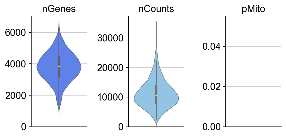
Note that in the preprocess stages, we calculate some basic statistics, the number of genes, total UMI counts and percentage of mitochondrial UMIs in each cell so we can visualize them via dynamo.pl.basic_stats(). Moreover, if the adata.var_name is not official gene names but ensemble gene ids, dynamo will try to automatically convert those gene ids into more readable official gene names.

dyn.pl.basic_stats(rpe1_kinetics,figsize=(2,3))

rpe1_genes = ['UNG', 'PCNA', 'PLK1', 'HPRT1']

rpe1_kinetics.obs.time

Cell_02365     15.0
Cell_02366     30.0
Cell_02367     30.0
Cell_02368     30.0
Cell_02369     45.0
              ...  
Cell_05418    120.0
Cell_05419    120.0
Cell_05420    180.0
Cell_05421    180.0
Cell_05422    180.0
Name: time, Length: 2793, dtype: float64

rpe1_kinetics.obs.time  = rpe1_kinetics.obs.time.astype('float')
rpe1_kinetics.obs.time = rpe1_kinetics.obs.time/60 # convert minutes to hours 

rpe1_kinetics.obs.time.value_counts()

time
0.50    574
0.75    564
0.25    442
2.00    408
1.00    405
3.00    400
Name: count, dtype: int64

Estimate time-resolved RNA velocity

There are some very non-trivial considerations between estimating time-resolved RNA velocity and estimating transcription/degradation kinetic rates. The following code provides the right strategy for time-resolved RNA velocity analysis using dynamo.tl.recipe_kin_data(). Wait for our final publication for more in-depth discussion of this interesting topic!

dyn.tl.recipe_kin_data(adata=rpe1_kinetics,
                       keep_filtered_genes=True,
                       keep_raw_layers=True,
                       del_2nd_moments=False,
                       tkey='time',
                      )

|-----> keep_filtered_cells_key is None. Using default value from DynamoAdataConfig: keep_filtered_cells_key=False
|-----> Running monocle preprocessing pipeline...
|-----------> filtered out 0 outlier cells
|-----------> filtered out 947 outlier genes
|-----> PCA dimension reduction
|-----> <insert> X_pca to obsm in AnnData Object.
|-----> computing cell phase...
|-----> [Cell Phase Estimation] completed [670.9501s]
|-----> [Cell Cycle Scores Estimation] completed [0.4995s]
|-----> [Preprocessor-monocle] completed [8.9135s]
|-----------> removing existing M layers:[]...
|-----------> making adata smooth...
|-----> calculating first/second moments...
|-----> [moments calculation] completed [26.3694s]
|-----? Your adata only has labeling data, but `NTR_vel` is set to be `False`. Dynamo will reset it to `True` to enable this analysis.
|-----> experiment type: kin, method: twostep, model: deterministic
|-----> retrieve data for non-linear dimension reduction...
|-----> [UMAP] using X_pca with n_pca_components = 30
|-----> <insert> X_umap to obsm in AnnData Object.
|-----> [UMAP] completed [17.9120s]
|-----> incomplete neighbor graph info detected: connectivities and distances do not exist in adata.obsp, indices not in adata.uns.neighbors.
|-----> Neighbor graph is broken, recomputing....
|-----> Start computing neighbor graph...
|-----------> X_data is None, fetching or recomputing...
|-----> fetching X data from layer:None, basis:pca
|-----> method arg is None, choosing methods automatically...
|-----------> method ball_tree selected
|-----> [calculating transition matrix via pearson kernel with sqrt transform.] in progress: 100.0000%|-----> [calculating transition matrix via pearson kernel with sqrt transform.] completed [3.8676s]
|-----> [projecting velocity vector to low dimensional embedding] in progress: 100.0000%|-----> [projecting velocity vector to low dimensional embedding] completed [0.9878s]
|-----> method arg is None, choosing methods automatically...
|-----------> method kd_tree selected

AnnData object with n_obs × n_vars = 2793 × 11522
    obs: 'Plate_Id', 'Condition_Id', 'Well_Id', 'RFP_log10_corrected', 'GFP_log10_corrected', 'Cell_cycle_possition', 'Cell_cycle_relativePos', 'exp_type', 'time', 'nGenes', 'nCounts', 'pMito', 'pass_basic_filter', 'total_Size_Factor', 'initial_total_cell_size', 'new_Size_Factor', 'initial_new_cell_size', 'Size_Factor', 'initial_cell_size', 'ntr', 'cell_cycle_phase'
    var: 'Gene_Id', 'nCells', 'nCounts', 'query', 'scopes', '_id', '_score', 'symbol', 'pass_basic_filter', 'log_m', 'score', 'log_cv', 'frac', 'use_for_pca', 'ntr', 'use_for_dynamics', 'use_for_transition'
    uns: 'pp', 'velocyto_SVR', 'feature_selection', 'PCs', 'explained_variance_ratio_', 'pca_mean', 'cell_phase_order', 'cell_phase_genes', 'vel_params_names', 'dynamics', 'neighbors', 'umap_fit', 'grid_velocity_umap'
    obsm: 'X_pca', 'cell_cycle_scores', 'X_umap', 'velocity_umap'
    varm: 'vel_params'
    layers: 'new', 'total', 'X_total', 'X_new', 'M_t', 'M_tt', 'M_n', 'M_tn', 'M_nn', 'velocity_N', 'velocity_T', 'cell_wise_alpha'
    obsp: 'moments_con', 'distances', 'connectivities', 'pearson_transition_matrix'

Visualize velocity streamlines

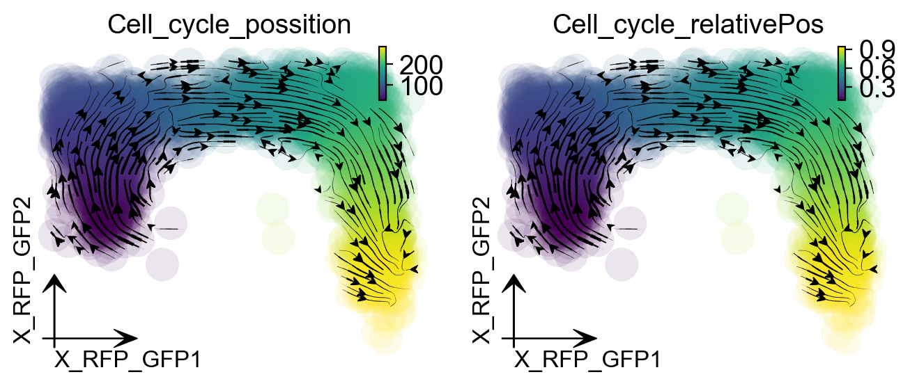
When we project our estimated transcriptomic RNA velocity to the space formed by the \(log_{10}(\) fluorescence\()\), Geminin-GFP and \(log_{10}(\) fluorescence\()\), Cdt1-RFP (Geminin and Cdt1 are two markers of different cell cycle stages), we can see a nice transition from early cell cycle stage to late cell cycle stage using dynamo.pl.streamline_plot().

def streamline(adata):
    dyn.tl.reduceDimension(adata, reduction_method='umap')
    dyn.tl.cell_velocities(adata, enforce=True, vkey='velocity_T', ekey='M_t', basis='RFP_GFP')
    dyn.pl.streamline_plot(adata, color=['Cell_cycle_possition', 'Cell_cycle_relativePos'], 
                           basis='RFP_GFP',figsize=(4,3))

    return adata

rpe1_kinetics.obsm['X_RFP_GFP'] = rpe1_kinetics.obs.loc[:, ['RFP_log10_corrected', 
                                                            'GFP_log10_corrected']].values.astype('float')
streamline(rpe1_kinetics)

|-----> retrieve data for non-linear dimension reduction...
|-----? adata already have basis umap. dimension reduction umap will be skipped! 
set enforce=True to re-performing dimension reduction.
|-----> [UMAP] completed [0.0027s]
|-----> [calculating transition matrix via pearson kernel with sqrt transform.] in progress: 100.0000%|-----> [calculating transition matrix via pearson kernel with sqrt transform.] completed [3.8565s]
|-----> [projecting velocity vector to low dimensional embedding] in progress: 100.0000%|-----> [projecting velocity vector to low dimensional embedding] completed [0.9468s]
|-----> method arg is None, choosing methods automatically...
|-----------> method kd_tree selected
|-----> method arg is None, choosing methods automatically...
|-----------> method kd_tree selected
|-----------> plotting with basis key=X_RFP_GFP
|-----------> plotting with basis key=X_RFP_GFP

AnnData object with n_obs × n_vars = 2793 × 11522
    obs: 'Plate_Id', 'Condition_Id', 'Well_Id', 'RFP_log10_corrected', 'GFP_log10_corrected', 'Cell_cycle_possition', 'Cell_cycle_relativePos', 'exp_type', 'time', 'nGenes', 'nCounts', 'pMito', 'pass_basic_filter', 'total_Size_Factor', 'initial_total_cell_size', 'new_Size_Factor', 'initial_new_cell_size', 'Size_Factor', 'initial_cell_size', 'ntr', 'cell_cycle_phase'
    var: 'Gene_Id', 'nCells', 'nCounts', 'query', 'scopes', '_id', '_score', 'symbol', 'pass_basic_filter', 'log_m', 'score', 'log_cv', 'frac', 'use_for_pca', 'ntr', 'use_for_dynamics', 'use_for_transition'
    uns: 'pp', 'velocyto_SVR', 'feature_selection', 'PCs', 'explained_variance_ratio_', 'pca_mean', 'cell_phase_order', 'cell_phase_genes', 'vel_params_names', 'dynamics', 'neighbors', 'umap_fit', 'grid_velocity_umap', 'grid_velocity_RFP_GFP'
    obsm: 'X_pca', 'cell_cycle_scores', 'X_umap', 'velocity_umap', 'X_RFP_GFP', 'velocity_RFP_GFP'
    varm: 'vel_params'
    layers: 'new', 'total', 'X_total', 'X_new', 'M_t', 'M_tt', 'M_n', 'M_tn', 'M_nn', 'velocity_N', 'velocity_T', 'cell_wise_alpha'
    obsp: 'moments_con', 'distances', 'connectivities', 'pearson_transition_matrix'

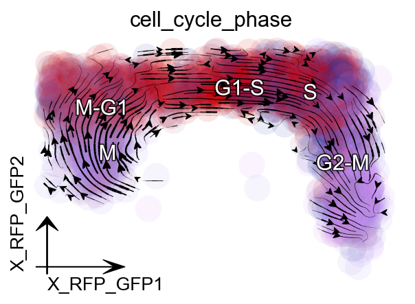
Since dynamo automatically performs the cell cycle staging at the preprocess step with cell-cycle related marker genes using methods from Norman et. al. We can also check whether dynamo’s staging makes any sense for this dataset. Interestingly, dynamo staging indeed reveals a nice transition from M stage to M-G, to G1-S, to S and finally to G2-M stage. This is awesome!

dyn.pl.streamline_plot(rpe1_kinetics, color=['cell_cycle_phase'], 
                       basis='RFP_GFP',figsize=(4,3))

|-----> method arg is None, choosing methods automatically...
|-----------> method kd_tree selected
|-----------> plotting with basis key=X_RFP_GFP
|-----------> skip filtering cell_cycle_phase by stack threshold when stacking color because it is not a numeric type

Animate cell cycle transition

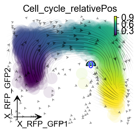
We use dynamo.vf.VectorField for vector field reconstruction and dynamo.pd.fate() for trajectory prediction to create an animation of cell cycle transition.

dyn.vf.VectorField(rpe1_kinetics, basis='RFP_GFP', 
                   map_topography=True, M=50)

|-----> VectorField reconstruction begins...
|-----> Retrieve X and V based on basis: RFP_GFP. 
        Vector field will be learned in the RFP_GFP space.
|-----> Generating high dimensional grids and convert into a row matrix.
|-----> Learning vector field with method: sparsevfc.
|-----> [SparseVFC] begins...
|-----> Sampling control points based on data velocity magnitude...
|-----> method arg is None, choosing methods automatically...
|-----------> method kd_tree selected
|-----> [SparseVFC] completed [0.1052s]
|-----------> current cosine correlation between input velocities and learned velocities is less than 0.6. Make a 1-th vector field reconstruction trial.
|-----> [SparseVFC] begins...
|-----> Sampling control points based on data velocity magnitude...
|-----> [SparseVFC] completed [0.0527s]
|-----------> current cosine correlation between input velocities and learned velocities is less than 0.6. Make a 2-th vector field reconstruction trial.
|-----> [SparseVFC] begins...
|-----> Sampling control points based on data velocity magnitude...
|-----> [SparseVFC] completed [0.0489s]
|-----------> current cosine correlation between input velocities and learned velocities is less than 0.6. Make a 3-th vector field reconstruction trial.
|-----> [SparseVFC] begins...
|-----> Sampling control points based on data velocity magnitude...
|-----> [SparseVFC] completed [0.0793s]
|-----------> current cosine correlation between input velocities and learned velocities is less than 0.6. Make a 4-th vector field reconstruction trial.
|-----> [SparseVFC] begins...
|-----> Sampling control points based on data velocity magnitude...
|-----> [SparseVFC] completed [0.0567s]
|-----------> current cosine correlation between input velocities and learned velocities is less than 0.6. Make a 5-th vector field reconstruction trial.
|-----? Cosine correlation between input velocities and learned velocities is less than 0.6 after 5 trials of vector field reconstruction.
|-----> Mapping topography...
|-----> method arg is None, choosing methods automatically...
|-----------> method kd_tree selected
|-----> [VectorField] completed [1.3628s]

progenitor = rpe1_kinetics.obs_names[rpe1_kinetics.obs.Cell_cycle_relativePos < 0.1]
len(progenitor)

78

from matplotlib import animation
info_genes = rpe1_kinetics.var_names[rpe1_kinetics.var.use_for_transition]
dyn.pd.fate(rpe1_kinetics, basis='RFP_GFP', init_cells=progenitor, 
            interpolation_num=100,  direction='forward',
   inverse_transform=False, average=False)

AnnData object with n_obs × n_vars = 2793 × 11522
    obs: 'Plate_Id', 'Condition_Id', 'Well_Id', 'RFP_log10_corrected', 'GFP_log10_corrected', 'Cell_cycle_possition', 'Cell_cycle_relativePos', 'exp_type', 'time', 'nGenes', 'nCounts', 'pMito', 'pass_basic_filter', 'total_Size_Factor', 'initial_total_cell_size', 'new_Size_Factor', 'initial_new_cell_size', 'Size_Factor', 'initial_cell_size', 'ntr', 'cell_cycle_phase', 'control_point_RFP_GFP', 'inlier_prob_RFP_GFP', 'obs_vf_angle_RFP_GFP'
    var: 'Gene_Id', 'nCells', 'nCounts', 'query', 'scopes', '_id', '_score', 'symbol', 'pass_basic_filter', 'log_m', 'score', 'log_cv', 'frac', 'use_for_pca', 'ntr', 'use_for_dynamics', 'use_for_transition'
    uns: 'pp', 'velocyto_SVR', 'feature_selection', 'PCs', 'explained_variance_ratio_', 'pca_mean', 'cell_phase_order', 'cell_phase_genes', 'vel_params_names', 'dynamics', 'neighbors', 'umap_fit', 'grid_velocity_umap', 'grid_velocity_RFP_GFP', 'cell_cycle_phase_colors', 'VecFld_RFP_GFP', 'fate_RFP_GFP'
    obsm: 'X_pca', 'cell_cycle_scores', 'X_umap', 'velocity_umap', 'X_RFP_GFP', 'velocity_RFP_GFP', 'velocity_RFP_GFP_SparseVFC', 'X_RFP_GFP_SparseVFC'
    varm: 'vel_params'
    layers: 'new', 'total', 'X_total', 'X_new', 'M_t', 'M_tt', 'M_n', 'M_tn', 'M_nn', 'velocity_N', 'velocity_T', 'cell_wise_alpha'
    obsp: 'moments_con', 'distances', 'connectivities', 'pearson_transition_matrix'

import matplotlib.pyplot as plt 

fig, ax = plt.subplots(figsize=(4,3))
ax = dyn.pl.topography(rpe1_kinetics, basis='RFP_GFP',
                       color='Cell_cycle_relativePos', ax=ax, 
                       save_show_or_return='return', fps_basis='RFP_GFP')
ax.set_aspect(0.8)

|-----------> plotting with basis key=X_RFP_GFP

%%capture
instance = dyn.mv.StreamFuncAnim(adata=rpe1_kinetics, basis='RFP_GFP', 
                                 color='Cell_cycle_relativePos', ax=ax, fig=fig)

|-----? the number of cell states with fate prediction is more than 50. You may want to lower the max number of cell states to draw via cell_states argument.

import matplotlib
matplotlib.rcParams['animation.embed_limit'] = 2**64 # Ensure all frames will be embedded.

from matplotlib import animation
import numpy as np

anim = animation.FuncAnimation(instance.fig, instance.update, init_func=instance.init_background,
                               frames=np.arange(100), interval=100, blit=True)
from IPython.core.display import display, HTML
HTML(anim.to_jshtml()) # embedding to jupyter notebook.

Once Loop Reflect