Molecular Interaction: Temporal Dominant Regulatory Interactions

To obtain mechanistic insights into key regulatory motifs from different perspectives, we developed three complementary strategies: cell-wise, trajectory-wise and plane-wise analyses. In this tutorial, we will introduce approaches for gene network motif analysis and guide you to perform cell-wise analyses of SPI1-GATA1 network motif.

Import relevant packages

import warnings
warnings.filterwarnings('ignore')
warnings.filterwarnings("ignore", message="numpy.dtype size changed")

import dynamo as dyn

dyn.configuration.set_figure_params('dynamo', background='white')
dyn.pl.style(font_path='Arial')
dyn.get_all_dependencies_version()

%load_ext autoreload
%autoreload 2

Using already downloaded Arial font from: /tmp/dynamo_arial.ttf
Registered custom font as: Arial


 ███                               ████████        
█████   █████    █████    █████    ███   █████      
   ██████   ██████   ██████   ████████      ████ 
  ___                           ████            ███
 |   \ _  _ _ _  __ _ _ __  ___                 ███
 | |) | || | ' \/ _` | '  \/ _ \█████           ███ 
 |___/ \_, |_||_\__,_|_|_|_\___/█████       ████  
       |__/                        ███   █████     
Tutorial: https://dynamo-release.readthedocs.io/       
                                     █████

package	umap-learn	typing-extensions	tqdm	statsmodels	setuptools	session-info	seaborn	scipy	requests	pynndescent	pre-commit	pandas	openpyxl	numdifftools	numba	networkx	mudata	matplotlib	loompy	leidenalg	igraph	dynamo-release	colorcet	anndata
version	0.5.7	4.13.2	4.67.1	0.14.4	79.0.0	1.0.1	0.13.2	1.11.4	2.32.3	0.5.13	4.2.0	2.2.3	3.1.5	0.9.41	0.60.0	3.4.2	0.3.1	3.10.3	3.0.8	0.10.2	0.11.8	1.4.2rc1	3.1.0	0.11.4

adata_labeling = dyn.sample_data.hematopoiesis()

|-----> Downloading processed hematopoiesis adata
|-----> Downloading data to ./data/hematopoiesis.h5ad
|-----> File ./data/hematopoiesis.h5ad already exists.

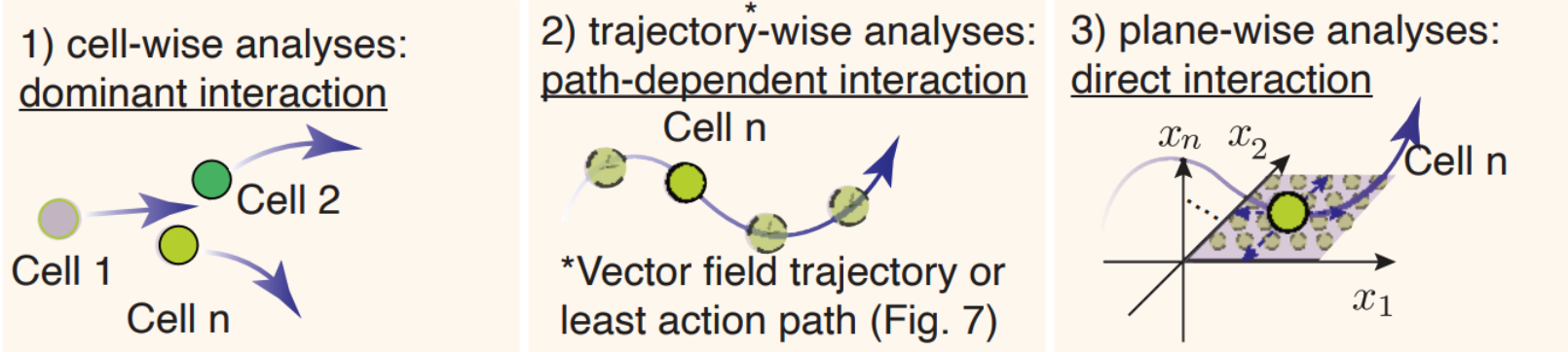
Three approaches for in-depth network motif characterizations

The schematic graph in this section shows the three approaches.

• cell-wise analyses to reveal dominant interactions across all cells

• trajectory-wise analyses reveal trajectory dependent interactions along a trajectory (predicted either from vector field streamline, or least action path, see Figure 6).

• Plane-wise analyses reveal direct interactions for any characteristic cell states by varying genes of interest while holding all other genes constant.

In the next section, we will use cell-wise analyses to analyze PU.1/SPI1–GATA1 network motif.

Cell-wise analyses of the PU.1/SPI1–GATA1 network motif across all cells

We showcase cell-wise analyses with the canonical PU.1/SPI1-GATA1 network motif.

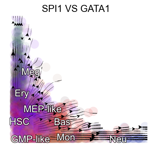
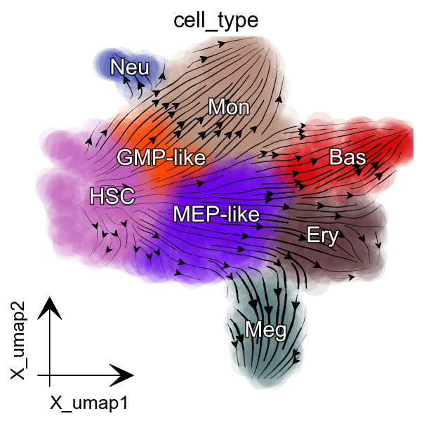
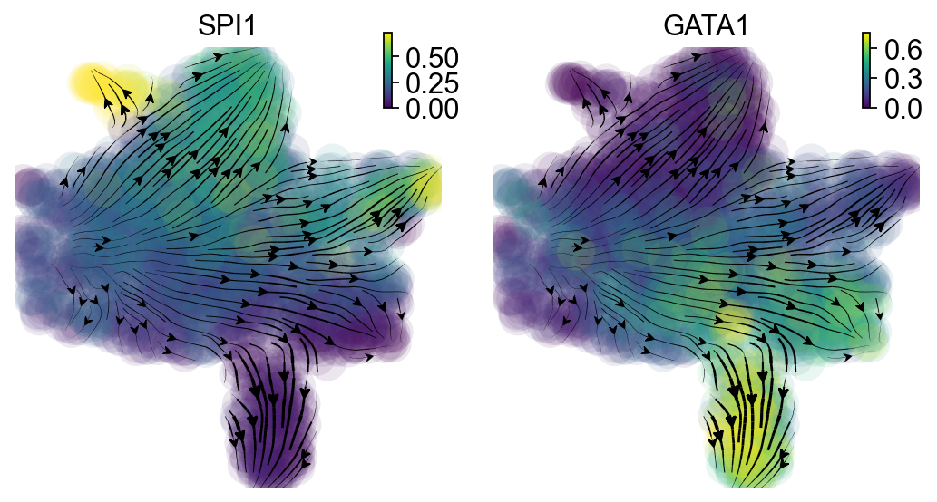
Streamline plot of the RNA velocities of SPI1 (x-axis) and GATA1 (y-axis)

The streamlines of SPI1 and GATA1 show that HSPCs bifurcate into GMP-like and MEP-like branches

#dyn.configuration.set_pub_style(scaler=4)
import matplotlib.pyplot as plt
fig, ax = plt.subplots(ncols=1, nrows=1, 
                       constrained_layout=True, 
                       figsize=(3, 3))
ax=dyn.pl.streamline_plot(
    adata_labeling,
    color="cell_type",
    x="SPI1",
    y="GATA1",
    layer="M_t",
    ekey="M_t",
    pointsize=0.5,
    ax=ax,
    vkey="velocity_alpha_minus_gamma_s",
    save_show_or_return='return',
    s_kwargs_dict={'adjust_legend':True,'dpi':80,
                  'arrow':False},
)

|-----> method arg is None, choosing methods automatically...
|-----------> method kd_tree selected
|-----------> plotting with basis key=X_umap
|-----------> skip filtering cell_type by stack threshold when stacking color because it is not a numeric type

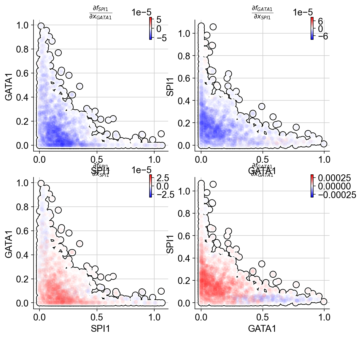
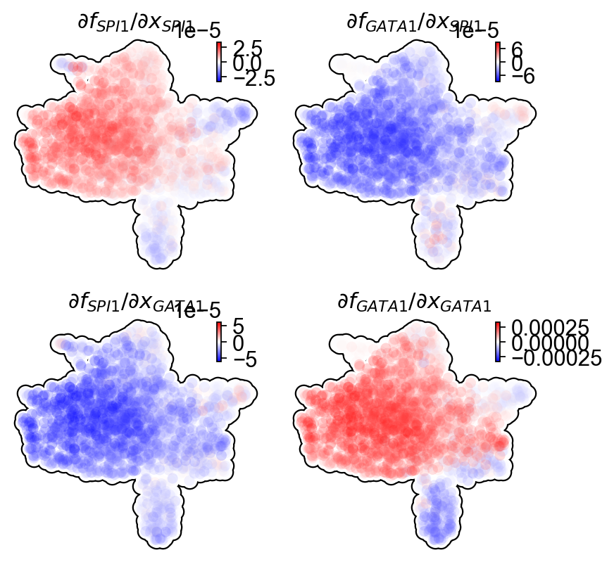
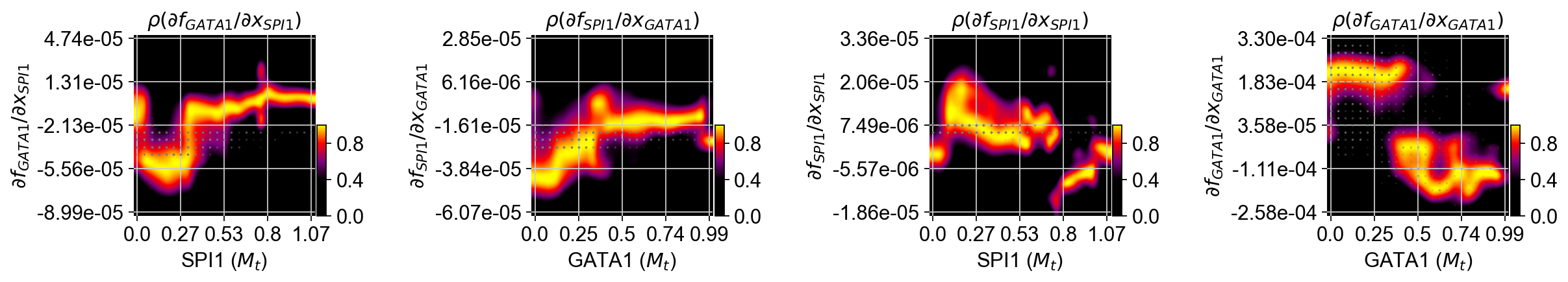
Next we will use jacobian to show

• Repression from SPI1 to GATA1, GATA1 to SPI1

• self-activation of SPI1, and GATA1, in the SPI1 and GATA1 expression space

In particular, the repression from SPI1 to GATA1 is mostly discernable in progenitors (rectangle A: bottom left) but becomes negligible when either GATA1 is much higher than SPI1 (rectangle B: upper left) or GATA1 is close to zero (rectangle C: bottom right).

%matplotlib inline
import numpy as np
genes = ["SPI1", "GATA1"]
def plot_jacobian_on_gene_axis(receptor, effector, x_gene=None, y_gene=None, axis_layer="M_t", temp_color_key="temp_jacobian_color", ax=None):
    if x_gene is None:
        x_gene = receptor
    if y_gene is None:
        y_gene = effector

    x_axis = adata_labeling[:, x_gene].layers[axis_layer].A.flatten(),
    y_axis = adata_labeling[:, y_gene].layers[axis_layer].A.flatten(),

    dyn.vf.jacobian(adata_labeling, regulators = [receptor, effector], effectors=[receptor, effector])
    J_df = dyn.vf.get_jacobian(
        adata_labeling,
        receptor,
        effector,
    )
    color_values = np.full(adata_labeling.n_obs, fill_value=np.nan)
    color_values[adata_labeling.obs["pass_basic_filter"]] =  J_df.iloc[:, 0]
    adata_labeling.obs[temp_color_key] = color_values

    ax = dyn.pl.scatters(
        adata_labeling,
        vmin=0,
        vmax=100,
        color=temp_color_key,
        cmap="bwr",
        sym_c=True,
        frontier=True,
        sort="abs",
        alpha=0.1,
        pointsize=0.1,
        x=x_axis,
        y=y_axis,
        save_show_or_return="return",
        despline=True,
        despline_sides=["right", "top"],
        deaxis=False,
        ax=ax,
        arrow=False,
    )
    ax.set_title(r"$\frac{\partial f_{%s}}{\partial x_{%s}}$" % (effector, receptor))
    ax.set_xlabel(x_gene)
    ax.set_ylabel(y_gene)
    adata_labeling.obs.pop(temp_color_key)

figure, axes = plt.subplots(2, 2, figsize=(8, 8))
plot_jacobian_on_gene_axis("GATA1", "SPI1", x_gene="SPI1", y_gene="GATA1", ax=axes[0,0])
plot_jacobian_on_gene_axis("SPI1", "GATA1", x_gene="GATA1", y_gene="SPI1", ax=axes[0,1])
plot_jacobian_on_gene_axis("SPI1", "SPI1", x_gene="SPI1", y_gene="GATA1", ax=axes[1,0])
plot_jacobian_on_gene_axis("GATA1", "GATA1", x_gene="GATA1", y_gene="SPI1",ax=axes[1,1])

|-----------> plotting with basis key=X_umap
|-----------> plotting with basis key=X_umap
|-----------> plotting with basis key=X_umap
|-----------> plotting with basis key=X_umap

The streamlines of SPI1 and GATA1 in UMAP space and colored by M_t show that HSPCs bifurcate into GMP-like and MEP-like branches clearly.

dyn.pl.streamline_plot(
    adata_labeling,
    color=["cell_type"],
    layer="M_t",
    figsize=(4, 4),
    ncols=2
)

dyn.pl.streamline_plot(
    adata_labeling,
    color=["SPI1", "GATA1"],
    layer="M_t",
    figsize=(4, 4),
    ncols=2,
    s_kwargs_dict={'adjust_legend':True,'dpi':80,
                  'arrow':False},
)

|-----> method arg is None, choosing methods automatically...
|-----------> method kd_tree selected
|-----------> plotting with basis key=X_umap
|-----------> skip filtering cell_type by stack threshold when stacking color because it is not a numeric type
|-----> method arg is None, choosing methods automatically...
|-----------> method kd_tree selected
|-----------> plotting with basis key=X_umap
|-----------> plotting with basis key=X_umap

UMAP jacobian analysis reveals self-activation of SPI1 in GMP and GATA1 in MEP, and mutual inhibition of SPI1 and GATA1 in GMP and MEP.

dyn.vf.jacobian(adata_labeling,
                regulators = ["SPI1", "GATA1"])
dyn.pl.jacobian(adata_labeling, figsize=(3,3),
                regulators = ["SPI1", "GATA1"])

Response heatmap

White dashed lines indicate the minimum or maximum of repression or activation and the corresponding expression threshold.

%matplotlib inline

dyn.vf.jacobian(adata_labeling, regulators=["SPI1", "GATA1"], 
                effectors=["SPI1", "GATA1"])
dyn.pl.response(
    adata_labeling,
    np.array([["SPI1", "GATA1"], ["GATA1", "SPI1"], 
              ["SPI1", "SPI1"], ["GATA1", "GATA1"]]),
    ykey="jacobian",
    log=False,
    drop_zero_cells=True,
    grid_num=25,
    figsize=(4, 3),
    save_show_or_return="show"
)

Conclusion

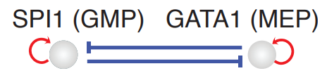
In the analyses above, we illustrate how to use dynamo to perform cell-wise analysis to explore the canonical PU.1/SPI1-GATA1 network motif. A schematic diagram of the SPI1-GATA1 toggle switch model can be summarized below.